Browser lab
The exercise and its data, running in a browser tab
This page holds the exercise of the course, Tasks 1 to 5, on a copy of R that runs inside the browser, with the data already in place and the same helper functions as the downloadable workspace. It is the page that the facilitator drives on the shared screen, a place to try the analysis and the data before you have installed anything, and the fallback for a machine that will not cooperate on the day. Everyone taking the course works in the downloadable workspace described on the Setup page. Nothing you do here is wasted, since both give the same numbers.
Five analysts reanalysed a claim from the EU-frames case (Teney 2016) for the Multi100 project (Aczel et al. 2026); you are analyst no. 6. Read the full task description, the claim, and the five-analyst table of findings on the Exercise overview page (the broader context of the project is set out in the course slides).
The five tasks take you from a setup check to two dots on the live class chart, one submitted while you explore the menu in Task 4 and one that you declare in your preregistration in Task 5 before running it.
Task 1 – Get yourself running
The aim of this task is only to reach the point where a line of R runs and the data are in front of you. Press Run Code on the cell below. If it prints the three lines it should, you are set up and everything else on this page will work.
You should see 270 rows, 27 countries and 10 years, and TRUE on the last line. If any of that is missing, reload the page and wait for the engine to finish downloading before pressing Run Code again. If it still fails, say STUCK in the chat.
Warm-up – the three R’s
The warm-up settles the vocabulary before you touch any data. Three of the four scenarios below describe one of our three R’s – reproducibility, robustness, replicability – and the fourth describes something else. Read all four, then label each one in the code cell.
Scenario 1: A reviewer reruns the authors’ Stata .do file on the authors’ data and gets a different coefficient from the one printed in the paper. This is an example of ______ even though what they tried to do failed.
Scenario 2: The analyst uses the authors’ submitted replication dataset, but they re-implement the model in R instead of Stata and centre the predictor. Is this a case of ______ or ______?
Scenario 3: A preregistered team tests the identical hypothesis on a separate, much larger dataset chosen to be theoretically equivalent, and gets results that contradict the original. Their conclusion is that the original analysis has failed to ______.
Scenario 4: Instead of the survey data used by the original authors, another researcher tests the same underlying idea on social-media texts using a machine-learning classifier method that the original never used. To their surprise, the authors’ original findings turn out to be ______, and the researcher concludes that they provide a reliable middle-range theory of the phenomenon they investigate.
Fill in the gaps in the code cell below and run it to print your answers back.
TipAnswers
- reproducibility – rerunning the same code on the same data. Here it failed to match, but the activity is still reproducibility, and ‘not reproduced’ is the verdict.
- arguably still reproducibility, in a grey area – re-implementing on the same data in different software is technically a re-computation – but centring the predictor nudges towards robustness. Two packages can also implement the same estimator differently, so make sure you know what the function you call is doing.
- replicability – same question, independent new data chosen to be theoretically equivalent.
- generalisability – the odd one out, with new data and a new method at once. It is the fourth cell of the matrix, outside the three that the exercise tests.
Task 2 – Meet the panel
The EU-frames dataset (EUframes_cy.csv) is already loaded for you as euframes. It is the country-year panel behind the whole exercise. The copy that this page loads is byte-identical to the one published in the analyst’s fork on OSF (osf.io/6zqct – “Multi100 | Teney_EurSocioRev_2016 | Analyst_C6HJR”, main folder), and the official Multi100 archival record is at osf.io/8rtwe. The downloadable workspace contains the same file.
Run the cell below to inspect the panel. Edit it freely – this is your environment.
You should see 270 rows, 27 countries, 10 years (2004–2013), and 13 columns. The outcome we care about first is mcosmo, the mean ‘cosmopolitan’ framing of the EU in each country-year, on a 0–1 scale. The predictor is unemp, the annual unemployment rate. growth is annual GDP growth, and n_cy is the number of survey respondents in each country-year. The codebook describes the other framings and every remaining column.
Now look at the outcome over time, one small panel per country:
In most countries the framing changes little over the decade, while in a few it moves sharply around the 2009 crisis. This variation within a country over time is what the fixed-effects model in Task 3 uses.
Task 2, continued – the estimand and the graph
Before fitting anything, say what you are trying to estimate, in words. A template you can adapt:
The unit-specific quantity is the change in mean cosmopolitan EU framing within a country-year associated with a one-point change in that country’s unemployment rate. The target population is EU member states over 2004–2013. The aggregation is the average of those unit-specific effects, holding fixed each country’s time-invariant traits and each year’s EU-wide shocks.
That last clause is a causal claim, and a directed acyclic graph makes it checkable. A DAG is a diagram of what causes what: variables are nodes, arrows run from cause to effect, and the rules for reading the graph then identify which variables have to be adjusted for if the arrow you care about is to be read cleanly. The graph below draws the five arrows that this exercise takes as given, which the rest of this page calls the committed arrows. Further down you decide which of the arguable arrows to add to them.
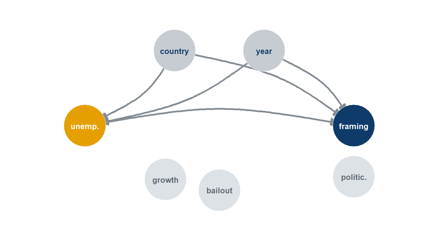
Five arrows are drawn. unemployment -> framing is the path of interest. Above it, country is a common cause of both: stable national traits such as size, EU tenure and labour-market institutions move local unemployment and shape how people frame the EU. year does the same job for the EU-wide shocks that hit every country in the same calendar year. The three pale nodes below have no arrows yet, because whether they belong is your decision.
You build the graph yourself in the cells below, in ordinary R. dagify() takes one formula per arrow, written the way you write a model, so framing ~ unemployment is the arrow that runs into framing. Read the tilde as ‘is caused by’ rather than ‘is regressed on’ and the direction comes out right every time. Because each arrow is its own line of R, an arrow you are unsure about can stay in the cell commented out, and adopting it means deleting a #.
dagify() and adjustmentSets() are already available on this page, so you can go straight to the next cell. The optional cell below adds the plot. It installs ggdag, which brings igraph, ggraph and four further dependencies with it – roughly 23 MB of download, and a noticeable pause on a slow connection. Run it if you want the plot. Skip it and everything else in Task 2 still works, because the figure above is the same graph.
Now specify the graph. The five committed arrows are live; the arguable ones are commented out, one substantive claim per line. Uncomment any you believe, then run the cell.
With the five committed arrows the minimal adjustment set is { country, year }, which is what a two-way fixed-effects model absorbs. An adjustment set is a set of variables that, once adjusted for, blocks every non-causal path from unemployment to framing, and it is minimal when no variable can be dropped from it without reopening one of those paths. Country fixed effects adjust for country and year fixed effects adjust for year, so the model that you will fit in Task 3 makes the same identification claim as the graph you have just written.
Now uncomment the growth pair and run the cell again. The set becomes { country, growth, year }, because a slump varies within a country over time and fixed effects only remove country-constant and year-common variation. The Task 3 model does not adjust for it, and your specification would need growth as a co-predictor to match your beliefs – a choice offered by the co-predictor axis of the menu in Task 5. The bailout arrows behave differently. A mediator lies on the path you are trying to measure, so the adjustment set does not grow when you add one; adjusting for it would remove part of the effect that you are trying to estimate.
Write two sentences for your own notes. What do two-way fixed effects adjust for, and what can they not fix? (Hint: anything time-varying within a country that you have not measured.)
Task 3 – Reproduce the recorded result
This is the reproducibility check. Fit the two-way fixed-effects model that follows from the constraints set by Multi100 for its second task:
mcosmo ~ unemp_c with fixed effects for country and yearwhere unemp_c is the unemployment rate centred on its grand mean. The target is t = −3.804 (df = 233, N = 270) – the value on record for analyst C6HJR in the Multi100 dataset.
The cell below is an exercise. Replace the blanks (______) with the missing code, then press “Run Code”. If you get stuck, open the hints below; the solution has the full code.
NoteHint 1 – centring
To centre a variable on its grand mean, subtract the mean of the whole column:
euframes$unemp_c <- euframes$unemp - mean(euframes$unemp)With fixed effects present this does not change the t-statistic, but the constrained specification includes it, so do it explicitly.
NoteHint 2 – the fixed-effects syntax
In fixest::feols, the bar | separates the regression from the fixed effects. To add country and year fixed effects, list them after the bar separated by +:
feols(mcosmo ~ unemp_c | cntry + year, data = euframes)
TipFully worked solution
euframes$unemp_c <- euframes$unemp - mean(euframes$unemp)
m1 <- feols(mcosmo ~ unemp_c | cntry + year, data = euframes)
broom::tidy(m1)
You should get estimate ≈ −0.00347, std.error ≈ 0.00091, statistic ≈ −3.80 – the recorded value reproduces from the published data and the published model. feols reports conventional (IID) standard errors by default when two fixed-effect dimensions are present, which is why it matches the plm value to three decimals.
NoteReproduction and the five analysts
You reproduced the recorded value, and so did everyone else in the class, because everyone ran the same code on the same file. This is why reproducibility is the cheapest of the three R’s to establish.
The five Multi100 analysts each wrote their own code for the same claim, and came back with five different answers, one of them not significant. Their pipelines are competent, well-organised work, so the spread is not a quality problem. It arises because a claim stated in words leaves several defensible quantities open, and different analysts estimate different ones without noticing that they have made a choice.
In Task 2 you named the quantity you are after and drew the graph from which your adjustment set follows. In Task 4 you find out how far the answer moves when the other choices change.
Task 4 – Work the menu
This task is exploratory. You try several specifications, look at what each one does, and get a feel for which choices move the estimate and which barely touch it. Nothing in this task is preregistered; the preregistration comes in Task 5.
try_spec() takes one argument per axis of the specification menu, and every argument defaults to the baseline that you have just reproduced. So changing one thing means changing one argument, and everything you do not name stays at baseline.
Each of the six calls below changes a single axis. The first four change the question that is being asked of the data; the last two keep the question and change only how it is measured. Run them and compare the results.
Then try your own combinations. The full set of arguments, with the baseline as the default for each:
Everything you try is logged. Print the log to see the small multiverse that you have just built. It shows only the axes that you varied, so the differences are easy to read:
When you have tried three or four, decide which one you would defend if you had to, run it once more so it is the most recent, and submit it. It appears on the live Multiverse chart as an exploratory result, marked with the tag that the cell prints, such as amber-otter-42. The tag is how you find your own circles on the chart, and your declared result in Task 5 carries the same one. To choose your own, write submit_exploration(nickname = "...") with a nickname rather than your name, because the chart is public:
NoteWhy ‘exploratory’?
Because you chose this specification after seeing what several specifications do, it lacks the guarantee that comes with a choice declared in a preregistration before its result is known – no one can rule out that it might have been chosen because of its result. This is something we almost never know in the case of published papers, unless their analysis has been preregistered and departures from the preregistration documented. In this course exploration is a natural step, and you also practise preregistering the analysis that you choose, so you submit twice, once here and once in Task 5.
Task 5 – Preregistration
Preregistration means setting out your choice in a plan before you see what it does, which stops you from quietly picking the specification that happens to give the answer you wanted. On this page the plan is the preregistration cell below, and it binds mechanically as well: the session remembers the choices that you declare in that cell, and every later cell reads them from there. The model builder refuses code that departs from them.
Make one choice on each of the fourteen axes of the specification menu, complete the dotted lines, then run the cell. The seven Level 1 choices fix the question you are asking, the four Level 2 choices fix how that question is measured, and the three Level 3 choices fix how it is estimated. Every axis is live. claim_align <- TRUE is the course convention, applied automatically: negative framings are reverse-coded (1 − y) and the claim-expected sign for growth is flipped, so ‘supports the claim’ reads as a negative sign for everyone.
An optional mirror form collects preregistrations from the class, and its link is shared in the session. It is not required. The cell above, copied into your notes, is your preregistration record.
Task 5, continued – build, run and report
This is the robustness check, and it is the part that your classmates cannot copy from you: together the class samples the multiverse of defensible analyses. You have declared your specification. Now translate it into model syntax yourself, filling the three gaps – the outcome, the right-hand side, and the estimator code – as you preregistered them. build_model() reads your declaration and accepts nothing else, and its error messages tell you what is off. Write the log form as log(unemp), and add any co-predictor with +.
NoteHint – from menu speak to model syntax
The formula uses the column names of euframes, with the outcome that you preregistered on the left of ~ and the predictor terms on the right. For the baseline declaration it is mcosmo ~ unemp. With the log form it would be mcosmo ~ log(unemp), and with a co-predictor mcosmo ~ unemp + growth. The estimator is the menu code itself, in quotes: "fe_twoway", "fe_country", "re" or "pooled_cl". You do not write the fixed-effects or clustering syntax here – the estimator code stands for it, and Task 3 showed what it expands to. Apart from the log form, the Level 2 and Level 3 choices never appear in the formula. They select which version of the panel the result was computed on and which fitting convention was used.
When the model is accepted, run it. Every specification on the menu is pre-computed. Six of the seven Level 1 choices name a small file that the page fetches from the site, and the other eight, which are the scoring rule and the seven Level 2 and Level 3 choices, pick one row inside it. These are the same numbers that a live fit produces, and you get them without downloading the estimation packages into your browser:
The output gives the coefficient, its claim-aligned partial r and your placement. The partial r is the correlation between predictor and outcome once the rest of the model is taken into account, and a value below zero supports the claim. The placement is the share of the grid of 840 specifications that supports the claim more strongly than your choice does. The five Multi100 analysts are placed between about the 16th percentile (the most strongly claim-supporting) and about the 68th (near the null).
Now send it to the class chart. The submission is built from your declaration, so there is nothing to fill in or transcribe. The cell prints your submission line and a pre-filled form link; click it and press Send. Your dot joins the live Multiverse chart within seconds, this time labelled declared and carrying the same tag as your exploratory result. If you have reloaded this page since Task 4, the session has forgotten that tag, so pass it back with report_result(nickname = "your-tag").
If the form will not open on your machine, read the printed numbers to the facilitator, who adds your dot to the chart.
If you want a second declared specification, edit the preregistration cell, rerun prereg(), rebuild and rerun. The chart will still label it declared, so be clear with yourself about what the second one is. Your first declaration was made without knowing its result. Anything after it was not, which puts it back in the same category as Task 4, and you should say so wherever you write about the result.
Taking it home
This page keeps nothing once you refresh it, so work you want to keep belongs in the downloadable workspace. Putting that work under version control and publishing the rendered report is the natural next step. The Git and GitHub self-study module explains it click by click.
References
Aczel, Balazs, Barnabas Szaszi, Harry T. Clelland, et al. 2026. “Investigating the Analytical Robustness of the Social and Behavioural Sciences.” Nature 652 (8108): 135–42. https://doi.org/10.1038/s41586-025-09844-9.
Teney, Céline. 2016. “Does the EU Economic Crisis Undermine Subjective Europeanization? Assessing the Dynamics of Citizens’ EU Framing Between 2004 and 2013.” European Sociological Review 32 (5): 619–33. https://doi.org/10.1093/esr/jcw008.