The statistical methods behind the course
From the linear model to meta-analysis
This is the statistics module of the companion curriculum. It works through the statistical methods that the EU-frames case draws on, from the simplest linear model to Bayesian and generalised extensions, using the course data throughout: the country-year panel you fit models on, the raw respondent-level records behind it, the specification grid behind the class chart, and the five Multi100 analysts whose results you meet on the day. It follows on from getting started with R and assumes only what that module covers – reading a CSV, a dplyr chain, and the idea of a model formula.
Every model on this page has been fitted, and every output shown comes from running it. The outputs come in two kinds. Models on the committed course data – the 270-row country-year panel and the small analyst and grid files – execute when this page is built, so what you see is what the code produces, and you can reproduce every one of them yourself from the shipped files. (The one exception is the Bayesian model of section 8: its data ship with the course too, but Stan compiles and samples for a minute or two, so its saved output is displayed instead, with the exact call that made it.) Models on the respondent-level microdata cannot ship, because the raw Eurobarometer records are GESIS-licensed and may not be redistributed. Those models were fitted once, on the facilitator’s machine, by the script companion/_model-outputs/fit_models.R in the source repository for the site, and their printed summaries are displayed here exactly as R returned them. The code above each such output is the code that produced it.
1. The country-year level
The original author (OA) modelled individual survey respondents directly. Sixteen Eurobarometer waves pool to 416,698 people interviewed across 27 EU member states between 2004 and 2013, each asked what the European Union means to them. The core exercise of the course works instead with EUframes_cy.csv, which collapses them to 270 country-year rows – 27 countries observed in each of 10 years – with every framing scale averaged within the cell. For country \(c\) in year \(t\), the cell value is the mean of its respondents’ scores:
\[ \bar{y}_{ct} = \frac{1}{n_{ct}} \sum_{i \,\in\, (c,t)} y_{ict} \]
where \(y_{ict}\) is respondent \(i\)’s framing scale and \(n_{ct}\) the number of respondents in that country-year. Unemployment and GDP growth, which are national figures to begin with, attach directly to each cell.
The data are therefore nested at three levels – respondents, country-years, and countries – and this module works through all three. Working at the middle level gains two things. The first is practical, and it is the reason that the course can exist at all: the raw microdata are GESIS-licensed and cannot be redistributed, whereas the derived country-year averages can be released under an open licence and shipped with the materials. The second is that the country-year is the level at which the predictor varies. Every respondent interviewed in Germany in 2010 shares one German 2010 unemployment rate, so all the information in the data about how unemployment and EU framing move together comes from 270 country-level pairings, however many individuals were interviewed. Aggregating to that level discards almost no identifying variation about the relationship of interest.
Averaging within a cell removes all the between-individual variation inside it, so nothing about how framing differs across people of different ages, educations or outlooks survives in the panel. The standard errors no longer reflect 416,698 respondents but 270 cells, which is why the fitted models below report residual degrees of freedom in the low hundreds rather than the hundreds of thousands. And a relationship among country-year averages need not hold among individuals: reading an aggregate association as if it described people is the ecological inference problem, and the country-year panel cannot be used to answer the individual-level question at all. Whether that matters depends on what you are trying to measure, the theme to which section 6 returns.
TipTry it
Read data/EUframes_cy.csv and sum its n_cy column (sum(euframes$n_cy)); you should recover the 416,698 respondents whose answers were averaged into the 270 rows. Then run nrow(euframes) to confirm the 270. Holding those two numbers side by side – the people who were interviewed and the rows you actually analyse – makes concrete what aggregation does.
2. The linear model
Every model in this module is a variation on one idea, so it pays to meet the idea in its plainest form. A linear model proposes that the outcome is a straight-line function of a predictor plus noise. For row \(i\) of the panel:
\[ y_i = \beta_0 + \beta_1 x_i + \varepsilon_i \]
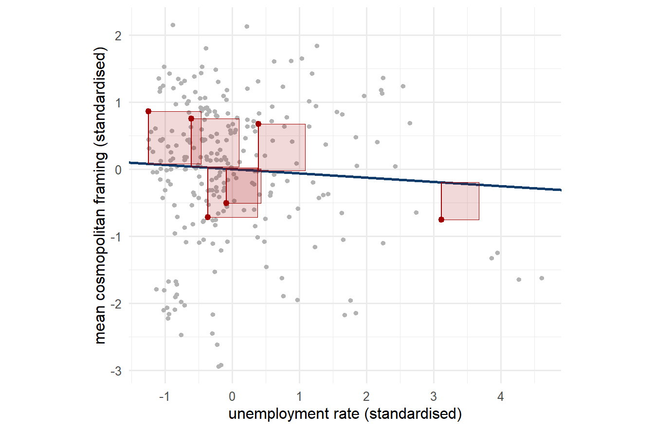
Each symbol has a plain meaning. \(y_i\) is the outcome, here the mean cosmopolitan framing score of a country-year. \(x_i\) is the predictor, its unemployment rate. \(\beta_0\), the intercept, is the expected outcome when the predictor is zero. \(\beta_1\), the slope, is the expected change in the outcome for a one-unit rise in the predictor, and it is the number on which every research question in this case depends. \(\varepsilon_i\) is the error: everything else that moves the outcome, assumed to average out to zero. Ordinary least squares (OLS) estimates the two \(\beta\)s by choosing the line that minimises the sum of squared errors,
\[ (\hat\beta_0, \hat\beta_1) = \underset{\beta_0,\,\beta_1}{\arg\min} \sum_i \left( y_i - \beta_0 - \beta_1 x_i \right)^2 \]
which is what lm() (for ‘linear model’) computes. The name ‘least squares’ is meant literally, as the figure below shows:
Nothing in that geometry is tied to a single predictor. Give the model two,
\[ y_i = \beta_0 + \beta_1 x_{1i} + \beta_2 x_{2i} + \varepsilon_i \]
and the fitted object is no longer a line but a plane floating over the grid of the two predictors. The errors are still the vertical gaps between each point and the fitted surface, OLS still minimises their summed squares, and each slope acquires the reading it keeps for the rest of this module: \(\beta_1\) is the expected change in the outcome for a one-unit rise in \(x_1\) with \(x_2\) held fixed, and ‘controlling for’ means no more than this movement along the plane parallel to one axis. The figure below fits this model on the panel, with GDP growth as the second predictor, the same variable that the specification menu can add as a co-predictor. It is a live three-dimensional object: drag it to rotate, scroll to zoom, and watch the red residual drops stay vertical from every angle.
null
1 With a third predictor the plane becomes a hyperplane that cannot be drawn, but the algebra in the arg-min never changes, and neither does the reading of a coefficient: each slope is a comparison with everything else in the model held level. The sections that follow stay with the single-slope version until the co-predictor choice on the menu brings growth back in.
The first argument of lm() is a formula, written outcome ~ predictor and read “outcome as explained by predictor”. The panel was read into euframes at the top of the page, this way:
library(readr)
euframes <- read_csv("../data/EUframes_cy.csv")   # ../ because this page lives in companion/
Fitting the model and reading it back takes two lines:
first_model <- lm(mcosmo ~ unemp, data = euframes)
summary(first_model)
Call:
lm(formula = mcosmo ~ unemp, data = euframes)

Residuals:
      Min        1Q    Median        3Q       Max
-0.208129 -0.036661  0.008259  0.051255  0.150833

Coefficients:
             Estimate Std. Error t value Pr(>|t|)
(Intercept)  0.516683   0.010133  50.989   <2e-16 ***
unemp       -0.001098   0.001055  -1.041    0.299
---
Signif. codes:  0 '***' 0.001 '**' 0.01 '*' 0.05 '.' 0.1 ' ' 1

Residual standard error: 0.07042 on 268 degrees of freedom
Multiple R-squared:  0.004025,  Adjusted R-squared:  0.0003084
F-statistic: 1.083 on 1 and 268 DF,  p-value: 0.299
This output format recurs, with variations, in every model that this module fits, so it is worth reading slowly once. The Call restates the model. The Residuals block summarises the estimated errors \(\hat\varepsilon_i = y_i - \hat y_i\), the gaps between each observed value and the fitted line. The Coefficients table contains the estimates themselves, one row per \(\beta\), four columns each:
- Estimate is \(\hat\beta\) itself. The
unemprow says a one-point rise in the unemployment rate goes with a fall of about 0.0011 in the cosmopolitan-framing score; the(Intercept)row says a hypothetical country-year with zero unemployment would be expected to score about 0.52. - Std. Error is the standard deviation of the estimate across imagined repeated samples: how precisely the data pin the coefficient down. It is the denominator of the
tvalue in the next column. - t value is Estimate divided by Std. Error – how many standard errors the estimate sits from zero. It is unit-free, which is why the course can put every submitted result on one chart: whatever the scale of the model, its
tmeans the same thing. - Pr(>|t|) is the p-value: the probability of a
tat least this large in magnitude if the true coefficient were zero. Small values are conventionally read as evidence that the association is not just noise.
Below the table, the residual standard error (0.070 here) estimates the spread of \(\varepsilon\), on 268 degrees of freedom (the 270 observations minus the two \(\beta\)s estimated). Degrees of freedom measure how many independent pieces of information remain for estimating uncertainty, and they matter repeatedly later in this module. Multiple R-squared is the share of the variance in the outcome that the line explains – 0.4% here, essentially nothing – and the F-statistic tests all the predictors at once.
Read as a whole, this first model finds no relationship worth reporting. The slope is small, its t of −1.04 is well inside the range that chance produces, and the p-value of 0.30 confirms it. Yet C6HJR’s published Multi100 coefficient, on exactly these 270 rows, is a clearly negative and conventionally significant t = −3.80. The data are identical in both fits, so the difference lies in the structure of the model, which the rest of this module works through.
The standard errors of OLS assume that the 270 errors \(\varepsilon_i\) are independent and identically distributed, and the estimate itself is only unbiased if the error is uncorrelated with the predictor. Both assumptions are strained here. The 270 rows are 27 countries observed ten times each, and the ten Danish rows share everything durable about Denmark. Those shared national features are part of \(\varepsilon\), they are correlated within country, and – since unemployment levels also differ durably between countries – they are correlated with \(x\) too. The next three sections deal with each consequence in turn: first the standard errors, then the estimate itself.
3. Clustered standard errors
Applied to a panel, the simple regression of section 2 has a proper name: pooled OLS, because it pools all country-years into one undifferentiated cloud. Writing the same equation with the two-index notation of the panel makes the pooling visible. One line serves every \(c\) and \(t\), and nothing in the model records that rows share a country:
\[ \bar{y}_{ct} = \beta_0 + \beta_1 x_{ct} + \varepsilon_{ct} \]
R offers several routes to this fit, and the course materials use three of them: lm() from base R, feols() from the fixest package (Bergé et al. 2026), and plm() from the plm package (Croissant and Millo 2023), the panel-econometrics toolkit that the published Multi100 analysis used. Before any new setting is introduced, a useful habit is to make different functions agree on the model you already understand. If two functions give the same numbers under settings you can name, you know what each is doing; when their defaults later diverge, you will know which setting moved.
library(fixest)
library(plm)

m_lm  <- lm(mcosmo ~ unemp, data = euframes)
m_fx  <- feols(mcosmo ~ unemp, data = euframes, vcov = "iid")
m_plm <- plm(mcosmo ~ unemp, data = euframes,
             index = c("cntry", "year"), model = "pooling")

tibble(
  fitted_with = c("lm()", "feols()", "plm()"),
  estimate  = c(coef(m_lm)["unemp"], coef(m_fx)["unemp"], coef(m_plm)["unemp"]),
  std_error = c(sqrt(vcov(m_lm)["unemp", "unemp"]),
                sqrt(vcov(m_fx)["unemp", "unemp"]),
                sqrt(vcov(m_plm)["unemp", "unemp"]))
)
# A tibble: 3 × 3
fitted_with estimate std_error
<chr> <dbl> <dbl>
1 lm() -0.00110 0.00105
2 feols() -0.00110 0.00105
3 plm() -0.00110 0.00105The three rows are identical to every digit, because they come from one estimator under three names: vcov = "iid" asks fixest for the classical standard errors that lm() and plm(model = "pooling") report by default. This like-for-like fit is the baseline, and the next step changes one setting only.
The first repair for the correlated-errors problem keeps the estimate and fixes the uncertainty. Cluster-robust standard errors replace the classical variance formula with one that permits the errors inside each cluster – here, each country – to be correlated in any pattern:
\[ \widehat{\operatorname{Var}}(\hat\beta) \;=\; (X'X)^{-1} \Big( \textstyle\sum_{g=1}^{G} X_g' \hat\varepsilon_g^{\vphantom{\prime}} \hat\varepsilon_g' X_g^{\vphantom{\prime}} \Big) (X'X)^{-1} \]
The notation is less fearsome than it looks. \(X\) is the matrix of predictor values and \(G\) the number of clusters (27 countries). The formula is a sandwich: the outer ‘bread’ terms are the ordinary OLS ingredients, and the middle ‘meat’ sums the residuals within each country in a way that keeps every within-country correlation intact instead of assuming it away. Only the standard error changes, and \(\hat\beta\) is untouched.
library(sandwich)
library(lmtest)

# fixest: one argument
m_cl <- feols(mcosmo ~ unemp, data = euframes, cluster = ~cntry)
coeftable(m_cl)
Estimate Std. Error t value Pr(>|t|)
(Intercept) 0.516683404 0.025017527 20.6528565 1.183841e-17
unemp -0.001097567 0.002195328 -0.4999559 6.213113e-01
attr(,"vcov_type")
[1] "Clustered (cntry)"# the same repair applied to the lm() fit via the sandwich package
coeftest(m_lm, vcov = vcovCL(m_lm, cluster = ~cntry, type = "HC1"))
t test of coefficients:

              Estimate Std. Error t value Pr(>|t|)
(Intercept)  0.5166834  0.0250175  20.653   <2e-16 ***
unemp       -0.0010976  0.0021953  -0.500   0.6175
---
Signif. codes:  0 '***' 0.001 '**' 0.01 '*' 0.05 '.' 0.1 ' ' 1
The two computations agree once the settings are matched. The default small-sample adjustment in fixest corresponds to type = "HC1" in sandwich (and to vcovHC(..., type = "sss") in plm). With type = "HC0" the numbers would drift apart in the trailing digits, the kind of discrepancy that the like-for-like habit is there to explain. Substantively, clustering doubles the standard error, and the t falls from −1.04 to −0.50, because the 270 rows were never 270 independent pieces of evidence.
Clustering cannot rescue the estimate, and here the pooled estimate itself is the problem. Because the model absorbs no between-country differences, its slope blends two different comparisons: how framing moves when unemployment rises over time within a single country, and how framing differs between high-unemployment and low-unemployment countries in the cross-section. In these data the two point in opposite directions. Section 5 puts numbers on them, about −0.0056 within countries and +0.0041 between. The pooled slope of −0.0011 is their blend, close to zero and, in many nearby specifications, on the wrong side of it.
This is the pattern that participants see on the class chart. Of the 140 specifications in the cosmopolitan universe (outcome = mcosmo), 41 come out with the ‘wrong’ sign, a positive coefficient running against the negative direction of the claim. Almost all of them come from one estimator:
| Estimator | Wrong-sign specifications (cosmopolitan universe) |
|---|---|
| Pooled OLS (cluster-robust) | 33 |
| Two-way fixed effects | 8 |
| Country fixed effects only | 0 |
| Random effects | 0 |
| Total | 41 |
Thirty-three of the 41 wrong-sign results are pooled models. The sign flip, in other words, comes overwhelmingly from throwing away the panel structure. Clustering is the right way to report uncertainty once you have chosen the pooled estimator; it does nothing to the sign, because the sign is a property of the estimate, not of its standard error.
TipTry it
Read data/spec_grid.csv, keep the cosmopolitan universe (filter(outcome == "mcosmo")), and count the wrong-sign specifications by estimator (filter(!supports_claim) |> count(estimator)). You should recover the 33-and-8 split in the table above. The count falls straight out of the committed grid, so you need not take the table on trust.
4. Fixed effects
The second repair goes after the estimate itself. C6HJR’s published Multi100 model, the one you reproduce in Task 3, is a constrained one: cosmopolitan framing regressed on the unemployment rate, with country and year fixed effects and nothing else.
\[ \bar{y}_{ct} = \beta\, x_{ct} + \alpha_c + \gamma_t + \varepsilon_{ct} \]
Here \(\alpha_c\) is a separate intercept for each country and \(\gamma_t\) a separate intercept for each year. The country effects \(\alpha_c\) absorb everything time-constant about a country – its language, institutions, size, and its enduring baseline level of EU enthusiasm – so the unemployment slope is identified only from how a country changes against itself over time, never from the fact that, say, Denmark and Greece differ. The year effects \(\gamma_t\) soak up everything common to all countries in a given year, the EU-wide shocks and the shared trajectory of the crisis among them. Two-way fixed effects therefore compare a country with itself over time, net of whatever moved all of Europe together in a given year.
Mechanically there are two equivalent ways to fit this, and comparing them shows how the estimator works. The literal way estimates every intercept, putting 26 country dummies and 9 year dummies alongside the slope, and is known as the ‘least squares dummy variable’ route. The efficient way never estimates them at all: the within transformation subtracts the mean of each country and the mean of each year from both sides,
\[ \left( \bar{y}_{ct} - \bar{y}_{c\cdot} - \bar{y}_{\cdot t} + \bar{y} \right) \;=\; \beta \left( x_{ct} - \bar{x}_{c\cdot} - \bar{x}_{\cdot t} + \bar{x} \right) + \tilde\varepsilon_{ct} \]
where a dot in place of an index means ‘averaged over it’. The demeaning wipes the \(\alpha_c\) and \(\gamma_t\) out of the equation, and OLS on the transformed data recovers exactly the same \(\beta\):
m_lsdv   <- lm(mcosmo ~ unemp + factor(cntry) + factor(year), data = euframes)
m_within <- plm(mcosmo ~ unemp, data = euframes, index = c("cntry", "year"),
                effect = "twoways", model = "within")
m_twfe   <- feols(mcosmo ~ unemp | cntry + year, data = euframes, vcov = "iid")

c(lsdv = coef(m_lsdv)["unemp"], plm = coef(m_within)["unemp"],
  feols = coef(m_twfe)["unemp"])
lsdv.unemp plm.unemp feols.unemp
-0.003472985 -0.003472985 -0.003472985 The three functions return one number because they fit one estimator. The fixest summary is the most informative of the three to read:
summary(m_twfe)OLS estimation, Dep. Var.: mcosmo
Observations: 270
Fixed-effects: cntry: 27, year: 10
Standard-errors: IID
Estimate Std. Error t value Pr(>|t|)
unemp -0.003473 0.000913 -3.80372 0.00018214 ***
---
Signif. codes: 0 '***' 0.001 '**' 0.01 '*' 0.05 '.' 0.1 ' ' 1
RMSE: 0.034875 Adj. R2: 0.715885
Within R2: 0.058465The slope is −0.00347: within a country, a one-point rise in unemployment goes with a fall of about 0.0035 in the mean cosmopolitan-framing score, net of common yearly shocks. Its t of −3.80 (p = 0.0002) is C6HJR’s published Multi100 coefficient. The two R-squared lines report different quantities. The overall adjusted R-squared of 0.72 mostly measures how much the fixed effects themselves explain – country identities are hugely predictive of framing levels – while the within R-squared of 0.058 is the contribution of the slope itself, with unemployment movements explaining about 6% of the within-country variation. Only the second bears on the research question.
The value recorded for analyst C6HJR in the Multi100 dataset is t = −3.804 (df = 233, N = 270), which is what this model returns and what the course reproduces in Task 3.
Two further points about that specification recur on the specification menu. First, grand-mean centring the predictor shifts the intercept but leaves the slope and its t untouched once fixed effects are present. A centred predictor and its raw form give an identical coefficient, which is why the specification grid keeps only the raw row and no redundant centred twin. Second, the standard error above is the classical one, matching the published analysis; ask fixest to cluster by country instead and the t of the same slope becomes −2.31 (p = 0.029). The result is still negative and still conventionally significant, but the shift shows that the uncertainty convention remains a separate and consequential choice even after the estimator is settled. When you compare outputs across analysts, check which convention each is reporting before comparing the ts.
What fixed effects cannot do is the reason that the course builds a causal graph before choosing a specification. They do nothing about time-varying confounding: anything that changes within a country over the period and moves both its unemployment and its EU framing – a national political scandal, a country-specific austerity programme, a swing in the governing party’s Europe stance – is not absorbed by either set of effects and can bias \(\beta\). Nor do they deal with feedback. If EU framing itself feeds back onto economic outcomes, or if both respond to some third time-varying driver, the model cannot detect it.
5. Within and between
Between the pooled and fixed-effects extremes sits a third estimator. Random effects keeps a country term in the model but, rather than estimating 27 separate intercepts, treats the country departures as draws from a distribution:
\[ \bar{y}_{ct} = \beta_0 + \beta_1 x_{ct} + u_c + \varepsilon_{ct}, \qquad u_c \sim N(0, \sigma_u^2) \]
Instead of 27 numbers, the model estimates a single one, the variance of the country effects \(\sigma_u^2\). Estimation is by generalised least squares, and its mechanics place the estimator on the spectrum that runs from pooled to fixed effects. Where fixed effects subtract the entire mean of each country, random effects subtract a fraction \(\theta\) of it:
\[ \bar{y}_{ct} - \theta \bar{y}_{c\cdot} = \beta_0 (1 - \theta) + \beta_1 \left( x_{ct} - \theta \bar{x}_{c\cdot} \right) + \text{error}, \qquad \theta = 1 - \sqrt{ \frac{\sigma_\varepsilon^2}{\sigma_\varepsilon^2 + T \sigma_u^2} } \]
with \(T\) the number of years per country. At \(\theta = 0\) this is pooled OLS, and at \(\theta = 1\) it is fixed effects. The data place it in between according to how much of the total variance lies between countries.
m_re <- plm(mcosmo ~ unemp, data = euframes,
            index = c("cntry", "year"), model = "random")
summary(m_re)
Oneway (individual) effect Random Effect Model
(Swamy-Arora's transformation)
Call:
plm(formula = mcosmo ~ unemp, data = euframes, model = "random",
index = c("cntry", "year"))
Balanced Panel: n = 27, T = 10, N = 270
Effects:
var std.dev share
idiosyncratic 0.001612 0.040151 0.337
individual 0.003170 0.056299 0.663
theta: 0.78
Residuals:
Min. 1st Qu. Median 3rd Qu. Max.
-0.1258 -0.0287 0.0014 0.0295 0.1275
Coefficients:
Estimate Std. Error z-value Pr(>|z|)
(Intercept) 0.55283984 0.01324871 41.7278 < 2.2e-16 ***
unemp -0.00525044 0.00081212 -6.4651 1.012e-10 ***
---
Signif. codes: 0 '***' 0.001 '**' 0.01 '*' 0.05 '.' 0.1 ' ' 1
Total Sum of Squares: 0.50821
Residual Sum of Squares: 0.43965
R-Squared: 0.13492
Adj. R-Squared: 0.13169
Chisq: 41.7974 on 1 DF, p-value: 1.0124e-10The Effects block is the new output to learn. The individual variance (0.0032) is \(\hat\sigma_u^2\), the between-country component, and the idiosyncratic variance (0.0016) is \(\hat\sigma_\varepsilon^2\), the within noise. The share column puts 66% of the error variance between countries. The reported \(\theta\) of 0.78 places this fit 78% of the way from pooled towards fixed effects, and the slope duly falls near the country-fixed-effects answer: −0.0053 (z = −6.5) against the −0.0056 that country fixed effects give on their own. (Note that the default random-effects model in plm has country effects only, so its natural comparator is one-way, not two-way, fixed effects.)
Random effects is more efficient than fixed effects when its central assumption holds: that the country effects \(u_c\) are uncorrelated with the predictor. Here that assumption is a strong one, because the unemployment level of a country is very likely tied up with the same durable national features that shape its baseline EU framing – the correlation that fixed effects were designed to remove. The Hausman test formalises the comparison. If the assumption held, fixed and random effects would estimate the same quantity and differ only by noise, so a large gap between them is evidence against it. Comparing the two one-way (country) estimators:
fe_country <- plm(mcosmo ~ unemp, data = euframes, index = c("cntry", "year"),
                  effect = "individual", model = "within")
re_country <- plm(mcosmo ~ unemp, data = euframes, index = c("cntry", "year"),
                  effect = "individual", model = "random")
phtest(fe_country, re_country)
    Hausman Test

data:  mcosmo ~ unemp
chisq = 9.8431, df = 1, p-value = 0.001705
alternative hypothesis: one model is inconsistent
The test rejects (p = 0.002). The estimators disagree by more than chance allows, so the random-effects assumption is not defensible here, and the fixed-effects estimate is the safer of the two.
A more informative response than picking a winner is to split the predictor into its two kinds of variation – the average unemployment of each country across the decade, and the departure of each year from that average – and give each its own slope. This is the within–between (or Mundlak) formulation:
\[ \bar{y}_{ct} = \beta_0 + \beta_W \left( x_{ct} - \bar{x}_{c\cdot} \right) + \beta_B\, \bar{x}_{c\cdot} + u_c + \varepsilon_{ct} \]
\(\beta_W\) is the within-country slope, \(\beta_B\) the between-country one. The fit below uses lmer() from lme4 (Bates et al. 2015), the standard R package for mixed models, which section 6 introduces properly. The random-intercept term (1 | cntry) plays the role of \(u_c\):
library(lmerTest)   # lmer() from lme4, plus degrees of freedom for its t-tests

euframes_wb <- euframes |>
  group_by(cntry) |>
  mutate(unemp_between = mean(unemp),
         unemp_within  = unemp - unemp_between) |>
  ungroup()

m_wb <- lmer(mcosmo ~ unemp_within + unemp_between + (1 | cntry), data = euframes_wb)
summary(m_wb)
Linear mixed model fit by REML. t-tests use Satterthwaite's method ['lmerModLmerTest']
Formula: mcosmo ~ unemp_within + unemp_between + (1 | cntry)
Data: euframes_wb
REML criterion at convergence: -862.4
Scaled residuals:
Min 1Q Median 3Q Max
-3.3294 -0.5742 0.0433 0.6396 3.0258
Random effects:
Groups Name Variance Std.Dev.
cntry (Intercept) 0.003170 0.05630
Residual 0.001612 0.04015
Number of obs: 270, groups: cntry, 27
Fixed effects:
Estimate Std. Error df t value Pr(>|t|)
(Intercept) 4.711e-01 3.664e-02 2.500e+01 12.857 1.61e-12 ***
unemp_within -5.645e-03 8.218e-04 2.420e+02 -6.869 5.42e-11 ***
unemp_between 4.143e-03 4.010e-03 2.500e+01 1.033 0.311
---
Signif. codes: 0 '***' 0.001 '**' 0.01 '*' 0.05 '.' 0.1 ' ' 1
Correlation of Fixed Effects:
(Intr) unmp_w
unemp_withn 0.000
unemp_betwn -0.953 0.000Read the two slopes against everything fitted so far. The within slope, −0.0056, is exactly the country-fixed-effects estimate (fit feols(mcosmo ~ unemp | cntry, ...) and compare), because separating out the between variation is what fixed effects do. The between slope is +0.0041, positive and imprecise. Countries with chronically higher unemployment do not frame the EU less cosmopolitanly, and if anything the pattern runs slightly the other way. The pooled puzzle of section 3 now has an arithmetic answer: the pooled slope of −0.0011 was a weighted blend of −0.0056 and +0.0041, two real patterns with opposite signs averaged into a figure close to zero. The Hausman test rejects for the same reason, because \(\beta_W \neq \beta_B\). The same comparison is a first encounter with the estimand, the quantity that an analysis sets out to estimate. ‘The effect of unemployment on EU framing’ has a within-country value and a between-country value, and choosing a model means choosing which of the two you are asking for. (For the fuller argument that this formulation should usually replace the fixed-versus-random contest, see Bell and Jones (2015).)
The random-effects estimator is also the reason that the grid holds 840 specifications rather than the full 960. Hold the outcome family at Gaussian and the predictor at unemployment, and the six remaining axes of the menu – six outcomes, two predictor forms, two co-predictor sets, four estimators, five samples and two weighting choices – multiply to 960. Frequency weights do not compose cleanly with the variance-component machinery that a random-effects GLS estimates, so the 120 weighted random-effects cells are omitted as not well defined. That arithmetic is all computable from the committed spec_grid.csv, as are the shares quoted from the grid: 68.7% of specifications in the direction of the claim and 63.9% significant.
6. Multilevel models
Every model so far has been fitted at the country-year level, whereas OA’s own study worked with individual respondents. Its published coefficient – b = −0.0034, t = −4.03, p < .001 (Table 3, Model 1) – comes from a three-level random-intercept model fitted to those respondents. This section moves down to that level and fits the same family of models on the actual microdata: 416,698 respondents, rebuilt from the sixteen GESIS waves as the codebook describes.
NoteHow the outputs in this section were produced
The respondent-level file cannot ship with the course (GESIS licence), so every model on this page that is fitted to it – the multilevel fits below and the generalised models of section 9 – is displayed rather than executed on the page. Each output was produced by the script companion/_model-outputs/fit_models.R in the repository for the site, run on the facilitator’s machine against the rebuilt person-level data. The text shown is verbatim R output. (The Bayesian summaries of section 8 come from the same script for a different reason: their model uses the committed panel, but compiling and sampling it takes a minute or two rather than the instant that a live chunk needs.) These are single, simple fits, chosen to teach how the output of each method is read. Other modules, among them the items module and the binary-outcomes module, fit further models to the same file and likewise display saved results. To run them yourself you need the raw waves under your own (free) GESIS registration – the data sources module walks through the registration.
A multilevel model (also called a hierarchical or mixed model) fits the respondents directly while representing the nesting explicitly: respondents within country-years, and country-years within countries. Written at its three levels, with \(i\) indexing respondents:
\[ y_{i(ct)} = \pi_{ct} + \varepsilon_{ict} \qquad\qquad \text{(respondents around their cell mean)} \] \[ \pi_{ct} = \alpha_c + \beta x_{ct} + r_{ct} \qquad \text{(cell means moved by unemployment)} \] \[ \alpha_c = \gamma_0 + v_c \qquad\qquad\quad \text{(countries around the grand mean)} \]
or, substituted into one line:
\[ y_{ict} = \gamma_0 + \beta x_{ct} + v_c + r_{ct} + \varepsilon_{ict} \]
with \(v_c \sim N(0, \sigma_v^2)\), \(r_{ct} \sim N(0, \sigma_r^2)\) and \(\varepsilon_{ict} \sim N(0, \sigma_\varepsilon^2)\). Three variance components now share the noise: \(\sigma_v^2\) for durable country differences, \(\sigma_r^2\) for country-year departures, and \(\sigma_\varepsilon^2\) for person-to-person differences inside a cell. The fixed part (\(\gamma_0 + \beta x_{ct}\)) is shared by everyone; the random part is a sum of draws at each level. This is the random-effects idea of section 5 generalised, and (1 | group) in lmer() notation declares each random intercept. The figure below draws the same structure:
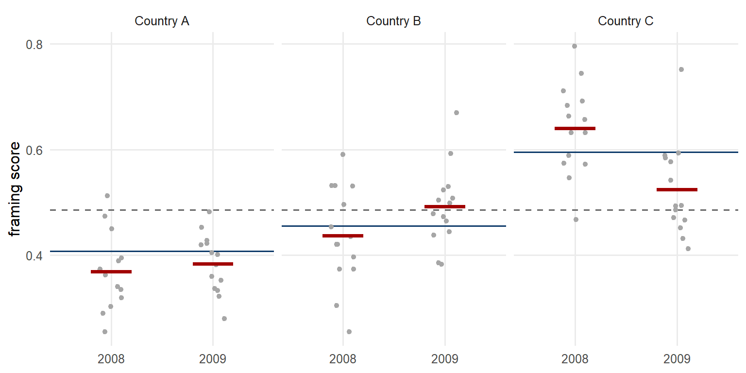
The first fit declares only the country level, which is too few levels for these data:
library(lme4)
person <- readRDS("data_private/eb_respondents.rds")   # 416,698 respondents, built by prep/01_build_respondents.R

m_two <- lmer(cosmo ~ unemp + (1 | cntry), data = person)
summary(m_two)
Linear mixed model fit by REML. t-tests use Satterthwaite's method ['lmerModLmerTest']
Formula: cosmo ~ unemp + (1 | cntry)
Data: person
REML criterion at convergence: 353436.4
Scaled residuals:
Min 1Q Median 3Q Max
-1.65509 -0.93396 0.00253 1.03162 1.80580
Random effects:
Groups Name Variance Std.Dev.
cntry (Intercept) 0.003941 0.06278
Residual 0.136677 0.36970
Number of obs: 416698, groups: cntry, 27
Fixed effects:
Estimate Std. Error df t value Pr(>|t|)
(Intercept) 5.474e-01 1.222e-02 2.705e+01 44.80 <2e-16 ***
unemp -4.790e-03 1.953e-04 3.912e+05 -24.52 <2e-16 ***
---
Signif. codes: 0 '***' 0.001 '**' 0.01 '*' 0.05 '.' 0.1 ' ' 1
Correlation of Fixed Effects:
(Intr)
unemp -0.140Read the output in two blocks. The Random effects block reports the estimated variance components (\(\hat\sigma_v^2 = 0.0039\) for countries, \(\hat\sigma_\varepsilon^2 = 0.1367\) for respondents), and the Fixed effects table reads like an lm() coefficient table with one addition – a df column, computed by Satterthwaite’s approximation, which estimates how many independent pieces of information support each t. That column shows the flaw in this model. A slope of −0.0048 with t = −24.5 on 391,200 degrees of freedom looks like overwhelming evidence, but the model has been allowed to treat every respondent as fresh information about unemployment, when every respondent in a country-year shares one unemployment value. The predictor has only 270 distinct values, so a model whose df runs to six figures is counting people as if they were countries.
Declaring the country-year level as well changes the result:
m_three <- lmer(cosmo ~ unemp + (1 | cntry) + (1 | cntry:year), data = person)
summary(m_three)
Linear mixed model fit by REML. t-tests use Satterthwaite's method ['lmerModLmerTest']
Formula: cosmo ~ unemp + (1 | cntry) + (1 | cntry:year)
Data: person
REML criterion at convergence: 350414.6
Scaled residuals:
Min 1Q Median 3Q Max
-1.77238 -0.96186 0.01493 0.99635 1.89818
Random effects:
Groups Name Variance Std.Dev.
cntry:year (Intercept) 0.001485 0.03853
cntry (Intercept) 0.003759 0.06131
Residual 0.135469 0.36806
Number of obs: 416698, groups: cntry:year, 270; cntry, 27
Fixed effects:
Estimate Std. Error df t value Pr(>|t|)
(Intercept) 5.526e-01 1.393e-02 4.441e+01 39.682 < 2e-16 ***
unemp -5.237e-03 8.021e-04 2.531e+02 -6.528 3.61e-10 ***
---
Signif. codes: 0 '***' 0.001 '**' 0.01 '*' 0.05 '.' 0.1 ' ' 1
Correlation of Fixed Effects:
(Intr)
unemp -0.502The slope barely moves (−0.0052), while its standard error quadruples, the t falls from −24.5 to −6.5, and the Satterthwaite df collapses from 391,200 to 253. That is the scale of the 270 cells, not of the 416,698 respondents, because the predictor varies only between cells. The new variance component (\(\hat\sigma_r^2 = 0.0015\)) is small in absolute terms, yet acknowledging it changes the inference fourfold. Set beside the aggregate models of section 5, the slope of −0.0052 (t = −6.5) from the three-level person model is, to two decimals, the aggregate random-intercept estimate. Once the error structure matches the real structure of the data, modelling 416,698 people and modelling their 270 cell means give the same answer about a country-year-level predictor – which is why the course can teach the case from the shipped panel.
The multilevel framework adds something new once more than the intercept is allowed to vary. A random slope lets each country have its own unemployment coefficient, drawn from a distribution whose spread is estimated:
\[ y_{ict} = \gamma_0 + (\beta + b_c)\, x_{ct} + v_c + r_{ct} + \varepsilon_{ict}, \qquad b_c \sim N(0, \sigma_b^2) \]
m_slopes <- lmer(cosmo ~ unemp + (1 + unemp | cntry) + (1 | cntry:year), data = person)
summary(m_slopes)
Linear mixed model fit by REML. t-tests use Satterthwaite's method ['lmerModLmerTest']
Formula: cosmo ~ unemp + (1 + unemp | cntry) + (1 | cntry:year)
Data: person
REML criterion at convergence: 350388.3
Scaled residuals:
Min 1Q Median 3Q Max
-1.76748 -0.95971 0.01417 0.99887 1.89847
Random effects:
Groups Name Variance Std.Dev. Corr
cntry:year (Intercept) 1.201e-03 0.034660
cntry (Intercept) 4.133e-03 0.064291
unemp 3.713e-05 0.006093 -0.44
Residual 1.355e-01 0.368061
Number of obs: 416698, groups: cntry:year, 270; cntry, 27
Fixed effects:
Estimate Std. Error df t value Pr(>|t|)
(Intercept) 0.553728 0.015552 20.196050 35.606 < 2e-16 ***
unemp -0.005712 0.001684 18.815257 -3.392 0.00309 **
---
Signif. codes: 0 '***' 0.001 '**' 0.01 '*' 0.05 '.' 0.1 ' ' 1
Correlation of Fixed Effects:
(Intr)
unemp -0.658In the Random effects block, the standard deviation of the slope is 0.0061, larger than the mean slope of −0.0057 itself. Countries do not share one unemployment effect. The model estimates that the effect ranges from clearly negative in some countries to positive in others, with the average lying where the earlier fits put it (the Corr of −0.44 adds that countries with higher intercepts tend to have more negative slopes). The df of the fixed slope is now about 19, because once each country contributes mainly to its own slope, the effective evidence for the average slope is the 27 countries, not the 270 cells. The df column tracks where the information comes from, and section 10 shows how much the converted effect sizes depend on it.
Two of the five Multi100 analysts worked at this level, and their results, once converted to partial correlations, mark the two ends of the range among the five. Analyst KEVF1 (in R) reported t = −5.90 with a Satterthwaite-style df of about 136, converting to a partial correlation of −0.452. Analyst PRL47 (in Stata) reported z = −3.59 with the respondent count of nearly 395,000 standing in for df, converting to −0.006. The two used the same data and the same model family and found the same negative direction, yet their converted effect sizes differ nearly 80-fold, almost entirely because of the df convention. Across the three model declarations above, the degrees of freedom moved from 391,200 to 253 to 19. The unit of analysis, and the error structure declared around it, is therefore an estimand choice: a decision about what ‘the effect’ refers to and which draws of the world would count as replications. The aggregated models answer a question about country-years. The person-level models appear to answer one about people, but with a predictor that varies only by country-year they mostly re-ask the same question with more elaborate error accounting. Reasonable analysts who answer ‘which question?’ differently get different numbers before any estimation begins.
Taking the grid arithmetic of section 5 down to the respondents shows, finally, what the framework means for the multiverse. Moving to the person level re-estimates the same 840 cells with more elaborate machinery, and it also widens the menu itself. Person-level covariates that simply do not exist in the aggregates – age, gender, education – become available as a new adjustment fork. The estimator axis changes membership: the multilevel designs of this section stand alongside their fixed-effects and pooled counterparts. The design weight attached to every respondent becomes usable at last (section 7), and with it one block of cells returns to the menu. The aggregate grid had to drop its 120 weighted random-effects cells because frequency weights do not compose with GLS, but genuine design weights do compose with multilevel models through the pseudo-maximum-likelihood route described in the weights module, so the weighted multilevel cells are well defined at the person level. Multiply the menu out – six outcomes, two predictor forms, two macro co-predictor sets, four estimators, five samples, two weight choices, and the new demographic-adjustment fork – and the person-level menu holds 1,920 Gaussian cells. Add the outcome-family choice that section 9 introduces, one more binary fork, and the universe doubles to 3,840 person-level specifications. Pooled with the family universe of 1,680 aggregated cells (the 840 of section 5 plus their family twins of section 9), they make a 5,520-specification joint universe in which the level of aggregation is itself a further fork, arguably the most consequential one on the whole menu. None of it has been computed. The arithmetic shows how a menu widens geometrically once the data allow new forks.
7. Survey weights
Every Eurobarometer respondent arrives with a design weight, the W1 weight that aligns each national sample with its population on sex, age, region and community size, and the person-level fits of section 6 have so far ignored it. Whether to use it is a decision of the same kind as the estimator choices above, and the weights module is where the course takes that decision apart: what the three kinds of weight on the specification menu are, which of them changes the estimand, how the survey package and WeMix fit a weighted model, why the same weighted multilevel model returns different numbers in different software, and what the two Stata analysts of the Multi100 study did about the design weights. The design-weighted fits – the pooled svyglm() and the two-level WeMix model, set beside the unweighted fit of section 6 – are in the estimation section of that module.
8. Bayesian estimation
Partial pooling – every random effect shrunk towards the grand mean by an amount that depends on how much data its group holds – is already half the Bayesian idea, and hierarchical models are the setting in which the full version is most useful. The shift is one of interpretation before machinery. Frequentist estimation asks ‘what parameter values make these data likeliest?’ and attaches uncertainty via imagined repeated sampling. Bayesian estimation treats the parameters themselves as uncertain quantities, starts from a prior distribution \(p(\theta)\) expressing what is plausible before the data, and updates it through the likelihood into a posterior:
\[ p(\theta \mid y) \;\propto\; p(y \mid \theta)\; p(\theta) \]
Everything you report – point estimates, intervals, probabilities of direction – is then read directly off the posterior distribution. For hierarchical models this has three practical consequences: the full uncertainty of group-level variances is kept even with few groups (our ten years are few), every derived quantity inherits that uncertainty instead of relying on a plug-in point estimate, and the assumptions that frequentist multilevel models make implicitly become stated priors that you can inspect and vary.
The likelihood \(p(y \mid \theta)\) is the model itself – the multilevel equations of section 6, read as a statement of how probable the observed data are under candidate parameter values. The prior \(p(\theta)\) says what is plausible for each parameter before the data arrive, which here means mild commitments such as ‘the between-country standard deviation is positive and probably not enormous’. Their product, renormalised, is the posterior \(p(\theta \mid y)\): a full probability distribution over all the parameters jointly, of which any coefficient table is only a summary. For real models that distribution has no closed form, so it is explored by sampling. Markov chain Monte Carlo draws thousands of parameter values whose long-run frequencies match the posterior, and the modern samplers (Hamiltonian Monte Carlo as implemented in Stan, which runs underneath everything below) have made this routine for the hierarchical models that this page has been building. Inference then is the summarising of draws: a posterior mean, an interval containing 95% of them, the share of them below zero. Two books suit a reader who wants to go further. Gelman and Hill’s classic (2007) leads from single-level regression to multilevel and Bayesian thinking. Its statistical chapters have aged well, though its software examples predate Stan and should not be typed in. McElreath’s Statistical Rethinking (2020) is the modern course-style introduction, and its examples exist in a free online translation into brms and tidyverse code (Kurz 2023) that pairs naturally with everything on this page.
The brms package (Bürkner 2017) makes the transition easy, because it accepts the same formula syntax as lmer(), translates the model to Stan, and estimates it by Markov chain Monte Carlo (MCMC) – four independent ‘chains’ of draws, whose agreement with one another is the convergence diagnostic. Here is the aggregate random-intercept model of section 5, now with a year intercept alongside, in its Bayesian form. This one uses the committed panel, so you can run it yourself. It compiles for about a minute and samples in seconds:
\[ \bar{y}_{ct} \sim N\!\left( \gamma_0 + \beta x_{ct} + v_c + w_t,\; \sigma^2 \right), \qquad v_c \sim N(0, \sigma_v^2), \quad w_t \sim N(0, \sigma_w^2) \]
library(brms)

m_bayes <- brm(mcosmo ~ unemp + (1 | cntry) + (1 | year), data = euframes,
               backend = "cmdstanr", chains = 4, iter = 4000, seed = 2026)
summary(m_bayes)
Family: gaussian
Links: mu = identity
Formula: mcosmo ~ unemp + (1 | cntry) + (1 | year)
Data: euframes (Number of observations: 270)
Draws: 4 chains, each with iter = 4000; warmup = 2000; thin = 1;
total post-warmup draws = 8000
Multilevel Hyperparameters:
~cntry (Number of levels: 27)
Estimate Est.Error l-95% CI u-95% CI Rhat Bulk_ESS Tail_ESS
sd(Intercept) 0.0627 0.0098 0.0471 0.0847 1.0028 1254 1945
~year (Number of levels: 10)
Estimate Est.Error l-95% CI u-95% CI Rhat Bulk_ESS Tail_ESS
sd(Intercept) 0.0184 0.0063 0.0094 0.0333 1.0020 1862 3555
Regression Coefficients:
Estimate Est.Error l-95% CI u-95% CI Rhat Bulk_ESS Tail_ESS
Intercept 0.5383 0.0157 0.5077 0.5691 1.0011 1019 1805
unemp -0.0036 0.0009 -0.0054 -0.0018 0.9998 5858 6558
Further Distributional Parameters:
Estimate Est.Error l-95% CI u-95% CI Rhat Bulk_ESS Tail_ESS
sigma 0.0378 0.0018 0.0345 0.0414 1.0005 4855 5142
Draws were sampled using sample(hmc). For each parameter, Bulk_ESS
and Tail_ESS are effective sample size measures, and Rhat is the potential
scale reduction factor on split chains (at convergence, Rhat = 1).The vocabulary of the output maps onto what you already know, though the meanings shift. Estimate is now the posterior mean and Est.Error the posterior standard deviation – the analogues of coefficient and standard error. The l-95% / u-95% CI columns are a credible interval, and unlike the confidence interval it means what everyone wants intervals to mean: given model and data, the parameter lies in this range with 95% probability. The genuinely new columns are the diagnostics. Rhat compares the four chains with one another. At convergence it is 1.00, and values above about 1.01 mean the sampler has not settled and the numbers should not be used. Bulk_ESS and Tail_ESS are effective sample sizes – how many independent draws the correlated MCMC samples are worth. The Multilevel Hyperparameters block shows what the Bayesian fit adds. sd(Intercept) for year is estimated at 0.018 with an interval running from 0.009 to 0.033, which states explicitly how little ten years of data can establish about a between-year variance, where a frequentist fit would give only a bare point estimate.
The slope itself, −0.0036, lies between the country-only random-effects estimate (−0.0053) and C6HJR’s two-way fixed-effects coefficient (−0.0035), because the year intercepts absorb the common yearly shocks much as the year fixed effects did. That placement is a property of the model, not of the Bayesian machinery, and the direct check is to fit the same model by REML – its exact frequentist twin, live on the committed panel:
m_freq_twin <- lmer(mcosmo ~ unemp + (1 | cntry) + (1 | year), data = euframes)
summary(m_freq_twin)$coefficients
Estimate Std. Error df t value Pr(>|t|)
(Intercept) 0.538805859 0.0147467137 54.01694 36.537351 9.024290e-40
unemp -0.003638517 0.0008628051 251.41246 -4.217079 3.455893e-05The result matches the displayed posterior within Monte Carlo error, with −0.0036 and a standard error of 0.0009 against a posterior mean of −0.0036 and an Est.Error of 0.0009. With 270 observations and weak priors, Bayesian and frequentist answers agree, as they should, because the data dominate. The two traditions come apart where data are thin, as the opening of this section anticipated, and the between-year variance is the place to compare them: REML gives a bare point estimate where the posterior gives a full interval.
The priors used by this model can be inspected, and inspecting them is a habit worth building:
prior_summary(m_bayes) prior class coef group resp dpar nlpar lb ub tag
(flat) b
(flat) b unemp
student_t(3, 0.5, 2.5) Intercept
student_t(3, 0, 2.5) sd 0
student_t(3, 0, 2.5) sd cntry 0
student_t(3, 0, 2.5) sd Intercept cntry 0
student_t(3, 0, 2.5) sd year 0
student_t(3, 0, 2.5) sd Intercept year 0
student_t(3, 0, 2.5) sigma 0
source
default
(vectorized)
default
default
(vectorized)
(vectorized)
(vectorized)
(vectorized)
defaultThe defaults in brms are mild: flat on the slope, a Student-t centred on the median of the data for the intercept, and half-Student-t distributions keeping the variance components positive but otherwise unconstrained. Priors are stated assumptions, which makes them open to argument. Re-fitting under different reasonable priors, as the course re-fits under different reasonable specifications, is the Bayesian form of the same robustness check. The person-level extension is a one-line change (the section 6 formula, data = person, and patience while 416,698 rows sample), and it leads into the generalised models of the next section.
9. Bounded outcomes
One assumption has gone unexamined since section 2: that a Gaussian linear model is the right shape for this outcome. Strictly, it never was. Every framing scale in this case is bounded between 0 and 1, whereas a Gaussian model has unbounded support. A straight line extended far enough therefore always predicts impossible values, and nothing inside lm() takes the bounds into account. The assumption is wrong at both levels of the data. What differs between the levels is how much that matters, as the two panels below show:
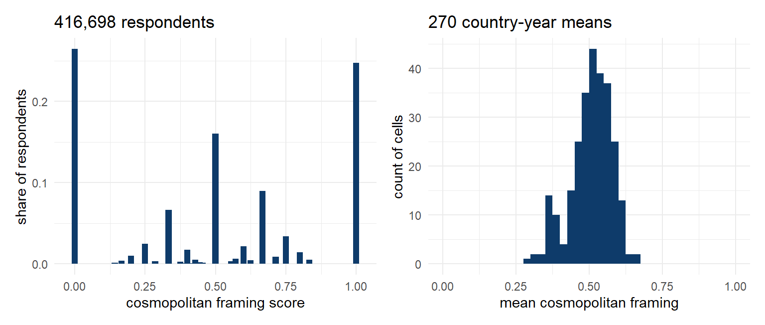
At the aggregate level (right panel) the cell means bunch in the middle of the scale, several residual standard deviations clear of either bound. Fitted values from the models of sections 2 to 5 never approach the bounds, the probability that the Gaussian error places beyond them is negligible, and the approximation is safe in practice, because of where this particular outcome happens to lie and not because the model allows for the bounds. That is a judgement to make consciously, and to re-make whenever an outcome drifts towards its floor or ceiling. At the person level (left panel) the judgement goes the other way. A respondent’s score is the share of their mentioned items that are cosmopolitan. A quarter of all respondents sit at exactly 0 and another quarter at exactly 1, and a Gaussian model treats those pile-ups as ordinary noise around a middle that describes almost nobody.
The generalised linear model (GLM) family fixes the shape problem by modelling a transformed mean:
\[ g\!\left( \mathbb{E}[y_i] \right) = \eta_i = \beta_0 + \beta_1 x_i \]
The linear predictor \(\eta_i\) stays a familiar straight line. The link function \(g\) maps the constrained mean of the outcome onto the unconstrained line, and a distribution suited to the actual support of the outcome replaces the Gaussian.
The classic member is logistic regression, for binary outcomes, with the log-odds link. Collapsing our outcome to ‘mentions at least one cosmopolitan item’:
\[ \log \frac{p_i}{1 - p_i} = \beta_0 + \beta_1 x_i, \qquad p_i = \Pr(y_i = 1) \]
m_logit <- glm(I(cosmo > 0) ~ unemp, family = binomial(), data = person)
summary(m_logit)
Call:
glm(formula = I(cosmo > 0) ~ unemp, family = binomial(), data = person)

Coefficients:
             Estimate Std. Error z value Pr(>|z|)
(Intercept)  1.262274   0.008360  151.00   <2e-16 ***
unemp       -0.026735   0.000837  -31.94   <2e-16 ***
---
Signif. codes:  0 '***' 0.001 '**' 0.01 '*' 0.05 '.' 0.1 ' ' 1

(Dispersion parameter for binomial family taken to be 1)

    Null deviance: 481477  on 416697  degrees of freedom
Residual deviance: 480478  on 416696  degrees of freedom
AIC: 480482

Number of Fisher Scoring iterations: 4
Reading the coefficients of a GLM takes one extra step, because the estimate is on the link scale. The slope of −0.027 is a change in log-odds per unemployment point; exponentiating gives an odds ratio of \(e^{-0.027} \approx 0.974\), and the quick ‘divide by four’ rule bounds the probability change at about −0.027 / 4 ≈ −0.7 percentage points per unemployment point at most. The z value replaces t (the dispersion is fixed, not estimated) and deviance replaces R-squared as the measure of fit. The z of −31.9 should now look suspicious, for the reason given in section 3. It comes from treating the 416,698 respondents as if each were fresh evidence about 270 unemployment values. The generalised and the multilevel extensions deal with separate problems, and this outcome needs both at once.
For a bounded continuous outcome the classical tool is beta regression, which models a variable on the open interval (0, 1) with a logit-linked mean and a precision parameter \(\phi\). For our variable its defect is the endpoint masses, because the beta distribution places no probability at exactly 0 or 1. The traditional workaround, nudging the data inward, is the kind of silent choice that this course sets out to make visible. Ordered beta regression (Kubinec 2023) builds the endpoints into the model. A single model uses ordered cutpoints to decide whether an observation is exactly 0, in between, or exactly 1, with a beta distribution for the middle, and one coefficient vector governs all three parts, so the slope keeps a single interpretation.
Both inferential traditions, frequentist and Bayesian, implement it. The frequentist route is glmmTMB (Brooks et al. 2017), a fast maximum-likelihood engine for GLMs with random effects – here with the full three-level structure of section 6, on all 416,698 respondents:
library(glmmTMB)

m_ordfreq <- glmmTMB(cosmo ~ unemp + (1 | cntry) + (1 | cntry:year),
                     family = ordbeta(), data = person)
summary(m_ordfreq)
Family: ordbeta ( logit )
Formula: cosmo ~ unemp + (1 | cntry) + (1 | cntry:year)
Data: person
AIC BIC logLik -2*log(L) df.resid
683220.8 683297.4 -341603.4 683206.8 416691
Random effects:
Conditional model:
Groups Name Variance Std.Dev.
cntry (Intercept) 0.015782 0.1256
cntry:year (Intercept) 0.006162 0.0785
Number of obs: 416698, groups: cntry, 27; cntry:year, 270
Dispersion parameter for ordbeta family (): 9.28
Conditional model:
Estimate Std. Error z value Pr(>|z|)
(Intercept) 0.183815 0.028629 6.421 1.36e-10 ***
unemp -0.011789 0.001665 -7.080 1.44e-12 ***
---
Signif. codes: 0 '***' 0.001 '**' 0.01 '*' 0.05 '.' 0.1 ' ' 1The output is made of pieces you now recognise: variance components for the two grouping levels (on the latent logit scale, so not directly comparable with those of section 6), a dispersion parameter (\(\phi\) = 9.3, the beta precision), and a conditional-model slope of −0.012 on the logit scale with z = −7.1. The divide-by-four rule translates that slope to at most −0.3 percentage points of cosmopolitan share per unemployment point, the same order as every Gaussian estimate of it, now from a model whose predictions cannot leave the unit interval. The z is −7 rather than −32 because the random effects do the clustering work that the bare logistic model ignored.
The Bayesian route is ordbetareg, Kubinec’s own implementation of the model on top of brms (Kubinec 2023). The exhibit below runs on a random subsample of 20,000 respondents, because the full-data posterior would sample for hours and the purpose here is to show the shape of the output, not to produce a final estimate:
library(ordbetareg)

set.seed(2026)
person_sub <- slice_sample(person, n = 20000)
m_ordbayes <- ordbetareg(cosmo ~ unemp + (1 | cntry), data = person_sub,
                         true_bounds = c(0, 1), backend = "cmdstanr",
                         chains = 4, iter = 2000, seed = 2026)
summary(m_ordbayes)
Family: ord_beta_reg
Links: mu = identity
Formula: cosmo ~ unemp + (1 | cntry)
Data: data (Number of observations: 20000)
Draws: 4 chains, each with iter = 2000; warmup = 1000; thin = 1;
total post-warmup draws = 4000
Multilevel Hyperparameters:
~cntry (Number of levels: 27)
Estimate Est.Error l-95% CI u-95% CI Rhat Bulk_ESS Tail_ESS
sd(Intercept) 0.1305 0.0209 0.0962 0.1782 1.0051 647 1264
Regression Coefficients:
Estimate Est.Error l-95% CI u-95% CI Rhat Bulk_ESS Tail_ESS
Intercept 0.1508 0.0316 0.0894 0.2107 1.0163 464 1126
unemp -0.0078 0.0020 -0.0118 -0.0038 0.9998 4370 3540
Further Distributional Parameters:
Estimate Est.Error l-95% CI u-95% CI Rhat Bulk_ESS Tail_ESS
phi 9.2926 0.1278 9.0450 9.5445 1.0009 3555 2674
cutzero -0.9643 0.0170 -0.9976 -0.9314 1.0000 3123 3302
cutone 0.7709 0.0085 0.7543 0.7878 1.0002 3138 3064
Draws were sampled using sample(hmc). For each parameter, Bulk_ESS
and Tail_ESS are effective sample size measures, and Rhat is the potential
scale reduction factor on split chains (at convergence, Rhat = 1).The output combines section 8 with what came before, and it is best read diagnostics first. The Rhat of 1.016 for the intercept is above the 1.01 bar, so its chains have not fully settled. In a production analysis the response would be to sample longer before using that parameter. The slope, by contrast, is clean (Rhat at 1.00, effective sample sizes in the thousands), and its posterior – −0.008 on the logit scale, credible interval −0.012 to −0.004 – agrees with the full-data glmmTMB estimate while being less precise on a twentieth of the data. The extra distributional parameters of the ordered beta family complete the comparison. cutzero and cutone are the ordered cutpoints governing the exact-0 and exact-1 masses, and phi, the beta precision, is estimated at 9.29, where the maximum-likelihood fit in glmmTMB put it at 9.28 on all 416,698 respondents.
This model family matters because of the central finding of the course. The fork that moves the results in this case is the operationalisation of the outcome, and how you model the distribution of the outcome is part of that fork. Treat the family as one more binary fork, Gaussian versus beta, both defensible for a bounded scale, and every universe it touches doubles. For the aggregated grid the doubling has been computed. The committed data/spec_grid_family.csv holds the family universe of 1,680 specifications – the Gaussian grid of 840, imported verbatim, plus a beta twin of each – built by companion/_model-outputs/build_family_grid.R from the committed panel and grid alone. The family axis appears on the specification menu as a first-class axis, always with the note that it is a course extension and not part of the Multi100 menu.
A second extension applies the same reasoning to the predictor. Task 2 of the Multi100 project fixed unemployment as the measure of poor economic performance, but Task 1 shows that three of the five analysts, left free, chose GDP measures instead – and OA’s own operationalisation used both. The menu therefore includes GDP growth as a second predictor on which the claim can be tested: raw form, alone or beside unemployment as a co-predictor, 840 cells across both outcome families at the standard measurement settings, and two published series to measure it by. Only the raw form is fitted. Affine transforms – centring, z-standardising – rescale a coefficient without moving its t, p or partial correlation, so on an r-ranked curve they would only ever duplicate a point that is already there. That is why the grid of 840 keeps a single raw-and-log pair per specification rather than four affine variants, and it is also part of why the share of specification variance taken by the predictor-form fork is essentially zero. In the growth universe the direction agrees with the claim about as often as it does for unemployment (70.5%), but significance falls below half (46.9%).
The twins are plain logit-link beta regressions on the cell means, well defined because the 270 means lie strictly inside the unit interval, as the right panel above showed, with none of the endpoint masses that force the ordered-beta repair at the person level. betareg fits the pooled and fixed-effects designs, with the fixed effects as country and year dummies and the pooled errors cluster-robust by country. beta_family() from glmmTMB fits the random-effects design, and the weighted random-effects exclusion of section 5 is mirrored, 120 cells per family. A beta model reports a z statistic rather than a t, and that changes nothing downstream. The section 10 conversion \(r = z / \sqrt{z^{2} + \mathit{df}}\) takes a z in place of a t, as it did for analyst PRL47 in the Multi100 record, so every twin is placed on the common axis unchanged. The grid also evaluates the significance of each twin against the same t reference that its Gaussian sibling uses, a uniform rule that matters only in the third decimal place at 100-plus df. Both halves can be checked straight from the committed file:
read_csv("../data/spec_grid_family.csv", show_col_types = FALSE) |>
  group_by(family) |>
  summarise(specifications = n(),
            claim_direction = mean(supports_claim))
# A tibble: 2 × 3
family specifications claim_direction
<chr> <int> <dbl>
1 beta 840 0.710
2 gaussian 840 0.687The Gaussian half, which is the grid of 840, has 68.7% of specifications in the direction of the claim and 63.9% significant, and the beta half has 71.0% and 63.1%. The beta twin of C6HJR’s published Multi100 specification – mcosmo, raw predictor, no co-predictor, two-way fixed effects, all years, unweighted – estimates a logit-scale slope of −0.014 with z = −4.075, converting to a partial correlation of −0.258 against C6HJR’s Gaussian −0.242. The direction is the same, the result is still significant, and the estimate is slightly stronger. The pattern of wrong signs from section 3 reappears line for line. In the cosmopolitan universe each family holds exactly 41 wrong-sign specifications, 33 of them pooled and 8 two-way fixed effects. Run the ‘Try it’ count from section 3 on the family grid and the split repeats twice over.
At the person level the doubling exists only as arithmetic. Taking the family fork down a level requires one substitution, because the person-level scales place real mass on exact zeros: the beta likelihood is unavailable there, and a logit-link fractional-response binomial would stand in as the twin of each cell (reverse-coding stays exact, since the flip works through the same logit identity). That takes the person-level universe to 3,840 specifications and the joint universe to 5,520, none of it computed. Because universes grow geometrically, one defensible fork at a time, the discipline is to state in advance which forks you consider defensible and why – the job of a preregistration – instead of running the largest universe you can afford.
10. A common scale
The five Multi100 analysts fitted different models, in different software, at different levels of analysis, so their raw coefficients are not comparable: a Stata pooled coefficient, an R fixed-effects coefficient and a person-level multilevel coefficient are not the same kind of number. Researchers have used meta-analysis on this problem for a century, and its machinery is worth learning properly before turning to what Multi100 borrowed from it, not least because it is a model that this page has already fitted.
Meta-analysis starts from \(K\) estimates \(\hat\theta_k\), each with a known sampling variance \(v_k\) (from its standard error). The equal-effects model assumes one true value \(\theta\) behind them all and pools by inverse-variance weighting, so precise studies count for more:
\[ \hat\theta_{\text{EE}} = \frac{\sum_k \hat\theta_k / v_k}{\sum_k 1 / v_k} \]
The random-effects model drops the one-true-value assumption and lets the true effects themselves vary between studies:
\[ \hat\theta_k = \mu + u_k + e_k, \qquad u_k \sim N(0, \tau^2), \quad e_k \sim N(0, v_k) \]
Here \(\mu\) is the average true effect, \(\tau^2\) the between-study variance, and \(e_k\) the sampling error of each study. In the notation of section 6, a random-effects meta-analysis is a two-level multilevel model, with studies as level-2 units and random intercepts \(u_k\). The main difference is that the level-1 variances \(v_k\) are not estimated but known, imported from the standard error of each study. Heterogeneity statistics then quantify the between-study spread: \(\tau\) on the scale of the effect itself, Cochran’s \(Q\) as a test, and \(I^2\) as the share of total variability that is real between-study difference rather than sampling noise.
For correlations, the conventional pooling scale is Fisher’s z transformation, \(z = \operatorname{atanh}(r)\), whose sampling variance depends only on sample size, \(v = 1/(n - 3)\). The five analysts’ recorded partial correlations are in the committed analysts5.csv, so the standard tool – the metafor package (Viechtbauer 2010) – can run on them live:
library(metafor)

analysts <- read_csv("../data/analysts5.csv", show_col_types = FALSE) |>
  mutate(zi = atanh(r), vi = 1 / (n - 3))

ma_re <- rma(yi = zi, vi = vi, data = analysts, method = "REML", slab = analyst_id)
ma_re
Random-Effects Model (k = 5; tau^2 estimator: REML)

tau^2 (estimated amount of total heterogeneity): 0.0472 (SE = 0.0347)
tau (square root of estimated tau^2 value):      0.2172
I^2 (total heterogeneity / total variability):   99.97%
H^2 (total variability / sampling variability):  3250.05

Test for Heterogeneity:
Q(df = 4) = 31765.7952, p-val < .0001

Model Results:

estimate      se     zval    pval    ci.lb    ci.ub
 -0.2481  0.0991  -2.5035  0.0123  -0.4423  -0.0539  *

---
Signif. codes:  0 '***' 0.001 '**' 0.01 '*' 0.05 '.' 0.1 ' ' 1
As a demonstration this output repays reading line by line, but as an analysis it would be seriously wrong. Take the heterogeneity block first, where \(I^2\) reaches 99.97%. In a genuine meta-analysis that number would mean the studies barely share a phenomenon. Here its meaning is more specific, because we know that all five results come from the same data and claim. Sampling error explains essentially none of the spread between the five analysts. The spread is analytic variation, the product of choices about outcome, estimator, level and df, which is the subject matter of the multiverse expressed as a heterogeneity statistic. The pooled estimate, by contrast, should not be believed even as arithmetic, because meta-analysis assumes independent studies and five reanalyses of one dataset are the textbook violation. The weighting adds its own distortion. The two person-level analysts enter with \(v_k\) built from six-figure respondent counts, so the equal-effects pooled value (run method = "EE" yourself and it returns −0.17) is dominated by their two results and inherits the df problem examined in section 6. The Multi100 design borrowed the standardisation step of meta-analysis but not its pooling step, and it reports the distribution of results instead of an average that would assume independence.
The standard graphic of meta-analysis, the forest plot, shows the same thing:
forest(ma_re, atransf = tanh, refline = 0,
       xlab = "partial correlation r (back-transformed from Fisher's z)",
       header = c("Analyst", "r [95% CI]"))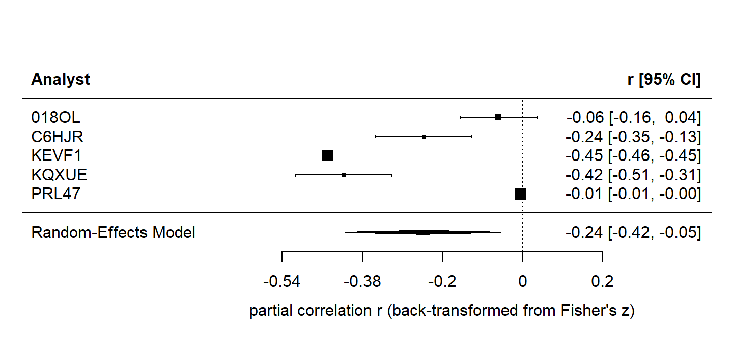
The five analysts
The five reanalyses answered a constrained brief. Task 2 of the Multi100 project fixed both ends of the question – use the positive non-materialist (cosmopolitan) form of EU framing as the outcome, use the unemployment rate as the measure of poor economic performance, and disregard the EU-policy and party-politicisation contextual variables of the paper – and left everything between them open. The table records what each analyst did with that freedom, as read from their public code:
| Analyst | Data as analysed | Outcome construction | Predictor | Controls | Estimator | SEs and df |
|---|---|---|---|---|---|---|
| 018OL | 420 country-by-wave cell means, EU-27 | mean of the 5 items, rescaled 0–1 | unemployment 15–74, raw | none | crossed random intercepts: country, year, EB wave | Satterthwaite, 396.9 |
| C6HJR | 270 country-years | cosmopolitan share, EU-frames panel | unemployment, centred | none | two-way FE: country + year | conventional, 233 |
| KEVF1 | 209,826 respondents | sum of the 5 items (0–7) | unemployment, raw | none | nested random intercepts: year within country | Satterthwaite, 135.6 |
| KQXUE | 270 country-years | cosmopolitan share | unemployment 20–64, raw | none | one-way country FE | conventional, 242 |
| PRL47 | 394,575 respondents | cosmopolitan share, no-opinion coded 0 | unemployment 25–64, raw + yearly change | gender, age, education, occupation, rural, crisis dummy, log GDP, growth | three-level: respondent in country-quarter in country | Wald z, no df |
That brief, though, belonged to the second of the two phases in the Multi100 design (Aczel et al. 2026). Task 1, months earlier, was free: analysts “could conduct and report as many analyses as they wished, but they had to draw a single conclusion”. The second table records what the analysts did in that free phase:
| Analyst | Free-phase predictor | Free-phase outcome | Recorded verdict |
|---|---|---|---|
| 018OL | GDP per capita (level, Eurostat) | positive framing, 7-item mean | evidence for the claim |
| KEVF1 | GDP growth (Eurostat) | positive framing, 7-item sum | evidence for the claim |
| PRL47 | log GDP + quarterly growth + crisis dummy | three positive-framing shares | evidence for the claim |
| KQXUE | GDP growth and unemployment (Eurostat) | cosmopolitan + utilitarian shares | evidence for the claim |
| C6HJR | GDP growth and unemployment (World Bank) | positive framing, 7-item share | evidence for the claim |
Three of the five never used the unemployment rate until the instructions named it, and most were not using the non-materialist outcome that the instructions fixed. Yet all five recorded the same categorical Task-1 verdict, because Task 1 asked for a conclusion, not a number – no standardised Task-1 effect sizes exist anywhere in the public Multi100 data. The instructions therefore created the common question that the standardised results answer. Read together, the two phases separate two robustness claims that are easily conflated: the five free analyses agreed in words, and the five standardised estimates, finally comparable, disagreed across a nearly 80-fold range. This course runs the sequence in reverse. Participants start from the standardised baseline and open one axis at a time, so on the day their freedom is structured as a menu of choices.
Every row of the standardised table is a defensible reading of the same brief, and the table explains the numbers that puzzle first-time readers. The Ns differ because the units differ. KQXUE and C6HJR collapsed respondents to 270 country-year means; 018OL kept the survey wave as its own grouping level, giving 420 country-by-wave cells; KEVF1 and PRL47 modelled respondents directly, and even their two Ns disagree because they prepared the data differently – KEVF1 merged an unemployment series with full country coverage only from 2009 (2004–2008 exists only for France), so complete-case fitting halved the stacked file to 209,826, while PRL47’s EU-27 filter and respondent-level controls left 394,575. The dfs then differ because each model counts the information about a country-year predictor in its own way. Fixed-effects OLS counts observations minus parameters, the Satterthwaite approximation estimates an effective df (397 on 420 cells, but 136 on 209,826 respondents, because the predictor varies only across country-years and the approximation takes this into account), and the mixed command in Stata reports an asymptotic z with no residual df at all. The conversion machinery below turns those choices into the numbers on the common axis.
In the standardisation step, every recorded result is converted to a partial correlation from just two numbers, the test statistic and its degrees of freedom:
\[ r = \frac{t}{\sqrt{t^{2} + \mathit{df}}} \]
Given the t (or z) and df of any model, it returns a number between −1 and 1, so that a Stata pooled model, an R fixed-effects model and every class submission can be read on one scale. This conversion produces the partial correlation that the course helpers submit_exploration() (Task 4) and report_result() (Task 5) send to the class chart on the Multiverse page, and it is why Task 2 of the Multi100 project asked every analyst for a statistic and its degrees of freedom in the first place. The closely related Cohen’s \(d\) follows from the same \(r\):
\[ d = \frac{2r}{\sqrt{1 - r^{2}}} \]
The same pair of numbers also gives the significance verdict, and that conversion belongs alongside the effect-size one because the two run in opposite directions. The two-sided p-value of a t statistic is the probability of a result at least as extreme when the true effect is zero – in R, 2 * pt(-abs(t), df). A z statistic runs the identical computation on the standard normal, 2 * pnorm(-abs(z)), which is simply the t-distribution with its df sent to infinity. That is why PRL47’s entry has no df. The df matters only at the margins here: with 20 df the 5% threshold is |t| = 2.09, and by a hundred df it has effectively converged on the normal value of 1.96. What matters far more is what each conversion does with the volume of data. The p-value asks whether the estimate stands out from zero given how much data went in, so at any fixed underlying effect it shrinks as n grows; the partial correlation divides the sample size back out. Given the same t and df, the two conversions can disagree sharply about which results are ‘big’, as the five analysts show:
| Analyst | Tool | Model unit | Statistic | df | p (two-sided) | N | Partial r |
|---|---|---|---|---|---|---|---|
| 018OL | R | aggregate | t = −1.21 | 396.9 | .229 | 420 | −0.060 |
| C6HJR | R | country-year (270) | t = −3.80 | 233 | < .001 | 270 | −0.242 |
| KEVF1 | R | person-level multilevel | t = −5.90 | 135.6 | < .001 | 209,826 | −0.452 |
| KQXUE | Stata | country-year (270) | t = −7.17 | 242 | < .001 | 270 | −0.419 |
| PRL47 | Stata | person-level multilevel | z = −3.59 | – | < .001 | 394,575 | −0.006 |
Every analyst found a negative effect, agreeing on direction, and four of the five clear the conventional significance bar decisively. Read the last two columns against each other, though, and the verdicts come apart. PRL47’s z of −3.59 is unambiguously significant (p < .001) while converting to a partial correlation of −0.006 – significance that comes from 394,575 respondents, not from the size of the effect. 018OL, the one non-significant row (p = .23), converts to an r ten times PRL47’s. A p-value and a standardised effect are answers to different questions, and neither substitutes for the other. Yet the partial correlations run from −0.006 to −0.452, a factor of about 75, and the two person-level analysts sit at the opposite extremes. The mechanism is the one traced through section 6. KEVF1’s conversion divides through a group-scale df of about 136, of the kind that the three-level and random-slope fits of section 6 produce; PRL47’s runs the respondent count through the denominator, of the kind that the two-level fit produced. The same negative relationship, converted under two df conventions, becomes either a substantial correlation or a rounding error. The course therefore insists on reading the degrees of freedom before the effect size, because a converted number is only as meaningful as the df behind it.
The common axis is also what makes the central result of the course legible. Decomposing the 840-specification grid to ask which analytical fork moves the estimate most gives this result:
| Analytical fork | Share of specification variance |
|---|---|
| Outcome (which framing scale) | ≈ 49.7% |
| Estimator + predictor form + co-predictor + weights (combined) | < 2% |
The choice of outcome – which of the four framing dimensions, or their positive and negative composites, you treat as ‘EU framing’ – accounts for roughly half of all the variation across the grid. Everything else that the menu lets you vary, the estimator choices of sections 3 to 6 included, together moves the result by under two per cent. That figure needs two qualifications. The decomposition is computed on the grid as estimated, before the claim-alignment convention that the course charts apply for display. Most of the outcome share is therefore the polarity split between positive and negative framings: real variation in what the specifications estimate, which the aligned chart removes from the picture but not from the decomposition. Recomputed on the claim-aligned scale in the facilitator’s extended analysis of the same grid, the ranking inverts, with the estimator fork rising to about 58% and the outcome fork falling to roughly 11–12%. Once every outcome points the same way, the pooled-versus-within contrast of section 5 becomes the largest source of variation. The outcome-family fork of section 9, meanwhile, barely registers: across the family universe of 1,680 rows the Gaussian-versus-beta choice accounts for under 1% of claim-aligned specification variance, and the two family curves all but coincide.
Under either decomposition, deciding what ‘EU framing’ means – which scale, and which polarity – sets what a model estimates before any of the estimation choices of sections 3 to 6 are made, and modelling the distribution of the outcome matters far less than choosing the outcome itself. For what a specification curve can and cannot conclude once all those results are on one axis, the course reading on the specification curve continues from this point.
Sources and provenance
This module was written from scratch for the course, and every number in it is computed, not quoted. The models of sections 2 to 5, the outcome-scale figure and family-grid summary of section 9, and the meta-analysis of section 10 execute on this page from the committed files (EUframes_cy.csv, analysts5.csv, spec_grid_family.csv, cosmo_dist.csv). The country-year construction and item definitions are in the data codebook. The person-level and Bayesian outputs of sections 6 to 9 were produced by companion/_model-outputs/fit_models.R in the source repository for the site, run against the person-level rebuild of the sixteen GESIS waves. The raw microdata are GESIS-licensed and are never distributed with the course – the data sources module explains the registration route. The Task-1 free-phase recipes and recorded verdicts in section 10 come from the public code of the five analysts and the public dataset of the Multi100 project (Aczel et al. 2026). The wrong-sign counts, the 840-versus-960 arithmetic, and the claim-direction and significance shares come from spec_grid.csv. The fork-importance decompositions (outcome ≈ 49.7% of specification variance as estimated, estimator ≈ 58% on the claim-aligned scale) come from the facilitator’s extended analysis of the same grid, and the 3,840- and 5,520-specification universes of sections 6 and 9 are menu arithmetic, not computed analyses. The exhibit fits on this page are illustrations of each method, and no other model on this page is fitted to the microdata.
The methods and software cited above are gathered in the reference list below: the panel estimators (Bergé et al. 2026; Croissant and Millo 2023), within–between modelling (Bell and Jones 2015), the multilevel workhorse (Bates et al. 2015), survey-weighted estimation, which section 7 leaves to the weights module (Lumley 2004; Rabe-Hesketh and Skrondal 2006; Carle 2009; Bailey et al. 2023; GESIS Eurobarometer Data Service, n.d.), Bayesian estimation and its textbooks (Bürkner 2017; Gelman and Hill 2007; McElreath 2020; Kurz 2023), the generalised models (Brooks et al. 2017; Kubinec 2023), and meta-analysis (Viechtbauer 2010).
References
Aczel, Balazs, Barnabas Szaszi, Harry T. Clelland, et al. 2026. “Investigating the Analytical Robustness of the Social and Behavioural Sciences.” Nature 652 (8108): 135–42. https://doi.org/10.1038/s41586-025-09844-9.
Bailey, Paul, Blue Webb, Claire Kelley, Trang Nguyen, and Huade Huo. 2023. WeMix: Weighted Mixed-Effects Models Using Multilevel Pseudo Maximum Likelihood Estimation. https://american-institutes-for-research.github.io/WeMix/.
Bates, Douglas, Martin Mächler, Ben Bolker, and Steve Walker. 2015. “Fitting Linear Mixed-Effects Models Using Lme4.” Journal of Statistical Software 67 (1): 1–48. https://doi.org/10.18637/jss.v067.i01.
Bell, Andrew, and Kelvyn Jones. 2015. “Explaining Fixed Effects: Random Effects Modeling of Time-Series Cross-Sectional and Panel Data.” Political Science Research and Methods 3 (1): 133–53. https://doi.org/10.1017/psrm.2014.7.
Bergé, Laurent R., Kyle Butts, and Grant McDermott. 2026. “Fast and User-Friendly Econometrics Estimations: The R Package Fixest.” arXiv Preprint arXiv:2601.21749, ahead of print. https://doi.org/10.48550/arXiv.2601.21749.
Brooks, Mollie E., Kasper Kristensen, Koen J. van Benthem, et al. 2017. “glmmTMB Balances Speed and Flexibility Among Packages for Zero-Inflated Generalized Linear Mixed Modeling.” The R Journal 9 (2): 378–400. https://doi.org/10.32614/RJ-2017-066.
Bürkner, Paul-Christian. 2017. “Brms: An R Package for Bayesian Multilevel Models Using Stan.” Journal of Statistical Software 80 (1): 1–28. https://doi.org/10.18637/jss.v080.i01.
Carle, Adam C. 2009. “Fitting Multilevel Models in Complex Survey Data with Design Weights: Recommendations.” BMC Medical Research Methodology 9 (1): 49. https://doi.org/10.1186/1471-2288-9-49.
Croissant, Yves, and Giovanni Millo. 2023. Panel Data Econometrics in R: The Plm Package. https://cran.r-project.org/web/packages/plm/vignettes/A_plmPackage.html.
Gelman, Andrew, and Jennifer Hill. 2007. Data Analysis Using Regression and Multilevel/Hierarchical Models. Cambridge University Press.
GESIS Eurobarometer Data Service. n.d. Weighting Overview (Standard and Special Eurobarometer). Accessed July 17, 2026. https://www.gesis.org/en/eurobarometer-data-service/data-and-documentation/standard-special-eb/weighting-overview.
Kubinec, Robert. 2023. “Ordered Beta Regression: A Parsimonious, Well-Fitting Model for Continuous Data with Lower and Upper Bounds.” Political Analysis 31 (4): 519–36. https://doi.org/10.1017/pan.2022.20.
Kurz, A. Solomon. 2023. Statistical Rethinking with Brms, Ggplot2, and the Tidyverse: Second Edition. https://bookdown.org/content/4857/.
Lumley, Thomas. 2004. “Analysis of Complex Survey Samples.” Journal of Statistical Software 9 (8): 1–19. https://doi.org/10.18637/jss.v009.i08.
McElreath, Richard. 2020. Statistical Rethinking: A Bayesian Course with Examples in R and Stan. 2nd ed. CRC Texts in Statistical Science. Taylor; Francis, CRC Press.
Rabe-Hesketh, Sophia, and Anders Skrondal. 2006. “Multilevel Modelling of Complex Survey Data.” Journal of the Royal Statistical Society: Series A (Statistics in Society) 169 (4): 805–27. https://doi.org/10.1111/j.1467-985X.2006.00426.x.
Viechtbauer, Wolfgang. 2010. “Conducting Meta-Analyses in R with the Metafor Package.” Journal of Statistical Software 36 (3): 1–48. https://doi.org/10.18637/jss.v036.i03.