This is the simulation module of the companion curriculum, and it is optional. Most quantitative pages on this site analyse data that came from the world; this module analyses data that came from a recipe we wrote ourselves, so that the answer is known before any model runs. That inversion, known as fake-data simulation, is a standard habit in applied statistics. Regression and Other Stories uses it constantly, on the argument that fitting models to data whose coefficients you planted yourself is how you learn what your models can and cannot recover (Gelman et al. 2020). The same habit underpins classroom practice (Gelman and Vehtari 2024) and the workflow literature, where experimentation on simulated data is one of the named components of model-building (Gelman et al. 2026).
The module teaches from a dataset built for the purpose. EUframes_person_full.csv is a simulated person-level companion to the EU-frames case – 41,660 synthetic respondents across the real 270 country-year cells, with the real macro variables attached. It contains all four framing dimensions and both composites, and every individual variable that the original author (OA) used, namely sex, age, education as both years and bands, an eight-category occupational position, urbanisation, and left-right self-placement.
First, no Eurobarometer respondent appears in it. The raw microdata behind the case are GESIS-licensed and cannot be redistributed in any form, including as samples or extracts (the data sources module explains that regime), so a person-level dataset that this site can legitimately ship has to be synthetic. What the licensed file supplied, read once and locally, is a set of summaries: marginal distributions, a correlation matrix, and the coefficients of a model of the survey instrument. Those are aggregate statistics of the kind that published appendices report, and they are committed as _model-outputs/joint_*.csv and _model-outputs/item_*.csv.
Second, and more useful for teaching, the recipe is known. Simulation studies call such a recipe the data-generating process, meaning the explicit rule by which every value was produced. Real data never comes with its rule attached, whereas simulated data is nothing but the rule, so any model fitted to it can be judged against an answer that is already known.
1. The recipe
The generator is _model-outputs/simulate_person_joint.R, a committed script that can be read alongside this page, and it works in two stages, one deciding who is in the sample and the other what they say.
Stage one: who. A respondent’s characteristics are one draw from a latent multivariate normal whose correlation matrix was estimated on the real respondents. Each observed variable is a monotone transform of one coordinate of that draw: sex and employment status by a threshold, urbanisation by cutpoints, age, education and left-right through their quantile functions. Any marginal distribution you like can be reproduced this way, and every pairwise association comes with it.
The associations matter as much as the marginals. An earlier version of this twin drew age, sex and education independently, which is the natural first step but ignores how they covary. In the real respondents, age correlates with being unemployed at -0.24 and with education at -0.14. A regression coefficient is a partial association, so it depends on how the variables covary; if the covariation is wrong, the coefficients come out wrong however carefully the effect of each variable was set.
Stage two: what they say. In the real survey a respondent hears a list of things that the EU might mean and names those that apply, and their dimension scores are the shares of their mentions falling to each dimension. The generator simulates that instrument rather than the four scores. Each of the thirteen items has a latent propensity
with \(\mathbf{x}_i\) the respondent’s characteristics, \(\alpha_{j(ct)}\) a shift for their country-year, and the thirteen residuals correlated with one another. That is a multivariate probit, a set of probit equations, one per item, whose error terms are allowed to correlate. Each of its three parts does a different job. \(\boldsymbol\beta\) records who says what, the correlated residuals capture the tendency of people who name one thing to name its neighbour as well, and \(\alpha\) sets the level for the country-year.
Simulating the instrument gives the shares their exact zeros and ones, makes them sum to one automatically, and lets each dimension respond through its own items.
bcoef |>slice_max(abs(estimate), n =6) |>mutate(estimate =signif(estimate, 3))
Occupation dominates that list, which is why the twin includes it. An earlier version left occupation out of the answer stage entirely – respondents had an occupation, but it had no bearing on what they said – and the result reproduced the macro slopes while getting two thirds of the coefficients in the model wrong. Section 2 describes how that was found.
The country-year shift. A dimension score is a share of a respondent’s own mentions, so raising the cosmopolitan items lowers every other dimension even with its own items untouched. There is no formula for the shift that produces a given set of cell means, so for each of the 270 country-years the generator solves four shifts by Newton iteration (a numerical search that corrects a guess step by step) against a fixed reference sample, until the expected dimension means match those in the panel to within 1e-4.
# A tibble: 6 × 11
  cntry  year   age edu3  ses          urban      cosmo  util  comm   lib unemp
  <chr> <dbl> <dbl> <fct> <fct>        <fct>      <dbl> <dbl> <dbl> <dbl> <dbl>
1 AT     2008    46 mid   manager      rural        0     0       0     0  4.13
2 BE     2005    45 low   retired      large_town   0.5   0.5     0     0  8.44
3 IT     2004    30 mid   manager      small_town   1     0       0     0  7.87
4 LT     2012    52 mid   unemployed   rural        0     0       0     0 13.4
5 LU     2010    53 low   white_collar large_town   0.6   0.4     0     0  4.36
6 SI     2010    36 mid   manual       rural        0     0       0     1  7.24
# The share columns are stored rounded to six decimals, so four of them can# drift from their sum: the identities need a tolerance, not ==.identities <- sim |>filter(cosmo + util + comm + lib >0) |>summarise(`dimensions sum to 1`=all(abs(cosmo + util + comm + lib -1) <5e-6),`pos + neg = 1`=all(abs(pos + neg -1) <5e-6),`share exactly 0`=mean(cosmo ==0),`share exactly 1`=mean(cosmo ==1))identities
# A tibble: 1 × 4
  `dimensions sum to 1` `pos + neg = 1` `share exactly 0` `share exactly 1`
  <lgl>                 <lgl>                       <dbl>             <dbl>
1 TRUE                  TRUE                        0.197             0.224
Among respondents who mention anything, 20% score exactly zero on cosmopolitan framing and 22% score exactly one – the latter because someone who mentions one item and finds it cosmopolitan scores 1 by construction. This is faithful to the real instrument, and it is the concrete reason that beta regression, which needs the outcome strictly inside the unit interval, cannot be used at person level while it can be used on country-year means. The statistical methods module states that constraint; here you can verify it.
2. Parameter recovery
The first thing to do with data whose recipe you know is to ask a model to find what the recipe planted. There are two such questions here, and they need keeping apart.
At cell level the planted value is the coefficient from the panel itself, because the generator solves each country-year until its expected dimension means match those in the panel. So a model fitted to the cell means of the twin should land where the same model fitted to the real panel lands.
Rising unemployment pushes framing away from both cosmopolitan and utilitarian terms and towards communitarian ones. Growth works differently, lifting utilitarian framing most, which makes sense because that dimension is built from the economic-prosperity and social-protection items. The pattern comes from the real panel, which the twin reproduces by construction.
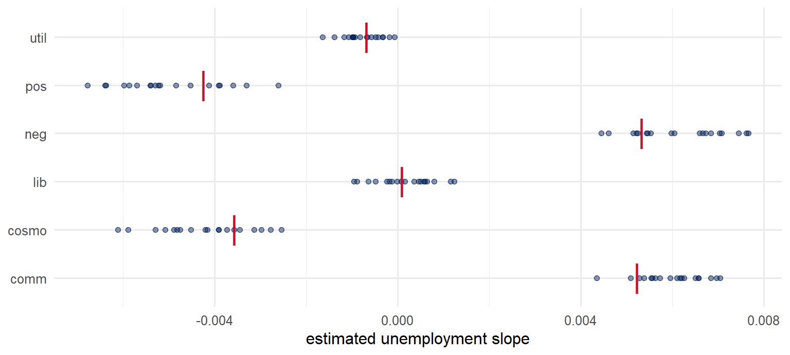
The simulated coefficients are close to the planted values without matching them, and the reason lies in the construction: each cell mean in the twin is an average over a tenth of the real respondents, so it is noisier than the corresponding mean in the panel. That noise is a property of the design, and it cannot be measured on a single dataset, because only repeated draws from the same recipe show how far the estimates scatter.
Figure 1: Independent draws from the same recipe, each refitted with C6HJR’s published Multi100 specification. Red marks show the planted coefficient. The unemployment slopes sit consistently outside their marks, which is the bias that the text discusses.
The last column is the test: each remaining gap as a multiple of the standard error of the mean across draws. 8 of the 12 fall inside two standard errors, and the ones outside are not scattered. Every unemployment slope misses in the same direction, with the estimate from the twin larger in magnitude than the planted value by 16 per cent at the median. The median is used because the planted slope of libertarian framing is nearly zero, so any absolute error there is an enormous proportion of it, and a mean would report a number driven entirely by the one quantity with almost nothing in it to estimate.
That is a real bias in the generator, and no single draw reveals it. Fit C6HJR’s published Multi100 specification to the committed twin and regress its cell means against those in the panel, and the unemployment coefficient on the difference comes back at t = −0.12, indistinguishable from zero. The sampling noise in one draw is the same size as the bias, so it takes a sweep of this size to separate the bias from zero.
The source is a documented limitation of the construction. The generator gives each country-year four numbers, one shift per dimension, where the real data has thirteen, one rate per item. A dimension-level shift captures as little as 37 per cent of the cell-to-cell variation in some items, and what is lost shows up twice over: as a mentioning rate about 1.6 points below the one in the panel, and as this amplification.
The obvious repair does not work. Giving each cell its own thirteen item rates makes the marginals exact – mentions per respondent come within 0.05 per cent of target – but makes the individual-level validation worse, from 39 coefficients agreeing to 32. In the real data the item rates of a cell reflect its context and the mix of people in it together. The twin draws its people from pooled marginals, so forcing the real rates onto a different mix pushes the difference into the country-year term, and it re-emerges as distorted covariate coefficients. Fixing it properly would mean reproducing the demographic composition of each cell as well, which is a much larger undertaking than the gain justifies.
The twin is therefore unbiased for the individual-level model that it was validated against, and biased by about a sixth for cell-level unemployment slopes. The cause of the bias is understood, and removing it was judged to cost more than it would gain.
At individual level the planted values are not those of the panel. They are whatever the real respondents give under the same model, so finding out whether the twin reproduces them means fitting that model on both files. That comparison is what licenses the twin to be used at all, and it is stored in _model-outputs/twin_validation.csv:
60 of 64 agree within two standard errors of the difference. The individual-level page interprets those coefficients.
The same validation found two real failures in earlier versions of this generator, and running the intended analysis on both files was the only check that detected them. The first version left occupation out of the answer stage, so a model containing occupation and education split the association between them differently from the real data – two thirds of the coefficients wrong, while every marginal, every cell mean and every correlation checked out. The second treated education as a straight line through a relationship that the published model represents in three bands, and returned about half of each band contrast.
TipTry it
Open the generator and change SIM_FRACTION from 0.10 to 0.40. That setting alone decides how many respondents each cell gets. The coefficients in the recipe stay as they are, so the only thing that changes is how precisely a cell mean can be measured.
Do not judge the result on one rerun, because a single draw gives one estimate, and one estimate cannot tell you whether the spread has narrowed. Sweep instead – ten seeds at each setting, with $SIM_SEED naming the draw and $SIM_SWEEP collecting the estimates – then compare the standard deviation of each set of ten. Quadrupling the cell sizes should roughly halve it, because the standard error of a mean falls with the square root of the sample size, and the sweep produces that rule as an experimental result. A simulation-based power analysis is built in the same way.
Point $SIM_OUT at a scratch directory unless you mean to overwrite the committed twin, and note that at 0.40 the file is four times the size.
3. The six outcomes
On the grid as estimated, the choice of outcome – which framing scale you treat as ‘EU framing’ – moves results more than any other analytical decision. The twin lets you see part of why, because the dimensions are shares of one instrument and cannot move independently.
On unemployment the signs follow the pattern that the claim-alignment convention of the course describes, with both positive framings declining as unemployment rises and both negative ones gaining. Growth does not follow the convention. There the cosmopolitan dimension moves with the communitarian one and utilitarian framing with the libertarian, so the split runs between whichever dimension is gaining and whichever are giving way, and which is which depends on the predictor. Libertarian framing is the weak case in that reading, since its growth coefficient is under one per cent of the communitarian one in size and what the two share is a sign rather than a magnitude. What claim alignment actually rests on is narrower and does hold exactly here: pos and neg partition the mentions, so neg = 1 − pos for every mentioner and reverse-coding the negative composite is exact arithmetic.
The magnitudes also span a wide range, so an analyst choosing util and one choosing comm are estimating genuinely different quantities from one instrument. The same spread is present in the real panel, and it is a substantial part of why the choice of outcome accounts for so much of the variation between specifications. The multiverse module takes that argument further, because this is where Auspurg’s objection about measurement nonequivalence applies.
4. Composition against context
The unemployment rate of a country-year could move EU framing in two ways. It might be that unemployed people frame the EU differently, so a high-unemployment cell holds more of them and its mean shifts with the mix – a compositional effect. Or living through high unemployment might change how everyone frames the EU, whatever their own situation. That would be a contextual effect.
The country-year panel cannot separate them, because it contains no individuals. This twin can, because it includes a calibrated occupational structure: being unemployed has its own estimated effect on what a respondent says, and the share of the respondents in a cell who are unemployed rises with the national rate by a measured amount.
Both halves matter, and the second is usually assumed without being measured. A large individual effect spread over a group that barely grows moves an average hardly at all, and the arithmetic that combines the two is more informative than either coefficient alone. The individual-level page does that calculation on this twin, and finds that the compositional path accounts for a few per cent of the country-level association.
An earlier version of this twin manufactured the compositional channel: it gave respondents an invented unemployment indicator whose prevalence was a fixed multiple of the national rate, so that this section would have something to display. Two things were wrong with that. Nothing about it was measured – the prevalence rule and the effect were both chosen. And it fused two constructs that belong to different levels, the unemployment rate of a labour market and the employment status of a person, which asserted a mechanism that the case never claimed and affected every unemployment coefficient that the twin planted.
A simulation can only demonstrate what was put into it. If the mechanism on display is one that you programmed into the generator yourself, the demonstration establishes only that your code works. Simulated data can therefore be used to check whether an estimator recovers an answer, but they cannot supply one.
5. Individual effects
The twin is built to reproduce the effects that age, sex, education, occupation and urbanisation have in the real respondents, which is what allows it to support the full published model. The table below compares each coefficient fitted on the real respondents with the same coefficient fitted on the twin.
Education is the largest individual effect in the file: graduates score about 0.12 higher on cosmopolitan framing than those who left school by fifteen, and the twin returns 0.10. The z column expresses each gap as a multiple of the standard error of the difference, so an absolute value below two means that the twin reproduces that coefficient as well as a second sample of its size would.
These individual coefficients are estimated much more precisely than the macro ones in section 2. Forty thousand respondents provide information about education, whereas only 270 cells provide information about unemployment. The same dataset is therefore highly informative about one question and weak on the other, a point about study design that section 9 develops.
TipTry it
Build your own placebo. Take any person-level variable in the file, shuffle it within country-year, and refit the model above with the shuffled version in place of the real one. Its coefficient should land near zero with an interval covering it, and if you repeat that twenty times, about one run in twenty will not, which is what a significance level of five per cent implies.
The placebo has to be a person-level variable. unemp, growth and bailout hold one value for a whole country-year, so shuffling them inside a cell puts every value back where it was and returns the real coefficient with the real p-value, which looks like a placebo that failed. A variable that does not vary within the unit you are permuting cannot be permuted there at all, and for the same reason a null cannot be built by shuffling within the level at which a macro predictor is measured.
6. Degrees of freedom
The statistical methods module presents a contrast that it can only display, because it rests on the licensed file. A naive analysis that ignores clustering reports an enormous t on hundreds of thousands of degrees of freedom, while the multilevel model reports a modest one on a couple of hundred, because the predictor varies only at the country-year level. On the twin you can run the contrast yourself.
m3 <-lmer(cosmo ~ unemp + (1| cntry) + (1| cntry:year), data = sim)naive <-lm(cosmo ~ unemp, data = sim)m3_par <- parameters::model_parameters(m3, ci_method ="satterthwaite")df_tbl <-tibble(model =c("naive OLS, clustering ignored", "three-level random intercepts"),estimate =c(coef(naive)[["unemp"]], fixef(m3)[["unemp"]]),se =c(sqrt(diag(vcov(naive)))[["unemp"]], m3_par$SE[m3_par$Parameter =="unemp"]),t = estimate / se,df =c(df.residual(naive), m3_par$df_error[m3_par$Parameter =="unemp"]))# The two rows differ in the estimate as well as in the standard error, so it is# worth having the within-country slope to hand: it is the one that the# multilevel fit leans towards, while the naive fit blends it with the# between-country one.cells_w <- sim_cells |>left_join(count(sim, cntry, year), by =c("cntry", "year"))B_WITHIN <-coef(lm(cosmo ~ unemp +factor(cntry), data = cells_w,weights = n))[["unemp"]]df_tbl |>mutate(across(where(is.numeric), \(x) signif(x, 3)))
# A tibble: 2 × 5
  model                          estimate       se     t    df
  <chr>                             <dbl>    <dbl> <dbl> <dbl>
1 naive OLS, clustering ignored -0.000555 0.000441 -1.26 41700
2 three-level random intercepts -0.00564  0.00108  -5.24   251
The naive row treats forty thousand respondents as independent pieces of evidence. The multilevel row counts only the few hundred effectively independent units, because respondents inside a country-year share one unemployment value and so provide largely overlapping information about it. Whenever the predictor is measured at a higher level, a person-level sample size suggests a precision that the design does not have. Respecting the structure costs degrees of freedom, and here it changes the estimate too: the naive fit is a different weighted average of between-country and within-country variation, landing at -5.55^{-4} against the multilevel -0.00564, which is close to the within-country slope of -0.00549. Neither of the two is the planted coefficient, because both leave out the year effects that C6HJR’s published Multi100 specification includes. This is also why, in Part 1 of the workshop, two Multi100 analysts fitting person-level models to the same claim could reach such different strengths of evidence.
7. Weights
Survey weights are usually taught as a procedure, but the question that matters in practice is when they change anything. Simulated data can answer it, because the distortion that the weight corrects can be built into the sample by design. The sample here was drawn with a fieldwork distortion – younger respondents over-selected – and w1 is the exact reciprocal of that selection factor, normalised to mean 1 within each country-year.
# Cell sizes are drawn in proportion to the real n_cy of each cell, so a person-level# mean over the respondents in the twin estimates the respondent-weighted value# in the panel. The average of the 270 cell means is a different quantity and# would make the weight look like it was doing harm.POP_COSMO <-weighted.mean(panel$mcosmo, panel$n_cy)ERR_UNW <-mean(sim$cosmo) - POP_COSMOERR_WTD <-weighted.mean(sim$cosmo, sim$w1) - POP_COSMOtibble(quantity =c("mean age", "mean cosmopolitan share"),unweighted =c(mean(sim$age), mean(sim$cosmo)),weighted =c(weighted.mean(sim$age, sim$w1),weighted.mean(sim$cosmo, sim$w1)),population =c(AGE_REF, POP_COSMO)) |>mutate(across(where(is.numeric), \(x) round(x, 3)))
# A tibble: 2 × 4
  quantity                unweighted weighted population
  <chr>                        <dbl>    <dbl>      <dbl>
1 mean age                    43.1     48.1         48.0
2 mean cosmopolitan share      0.479    0.471        0.5
The achieved sample is about four years too young, and weighting recovers the population age almost exactly. Because age affects framing in the recipe, that composition error propagates into the outcome: unweighted, the cosmopolitan share sits -0.021 above the population value, and weighting removes about -38 per cent of that. Weighting re-balances who is counted, so it matters only to the extent that the people who were over- or under-counted differ on the outcome.
The population column is itself a choice. A person-level mean over the respondents in the twin is aiming at the respondent-weighted value in the panel, not at the average of its 270 cell means, because cells enter the twin in proportion to how many real respondents they held. The two differ by 0.007, which is larger than the whole effect of the weight, so a table benchmarked against the wrong one would show weighting making the estimate worse. The choice of estimand, the quantity that a statistic is meant to estimate, therefore decides whether the table shows the weight helping or harming.
The distortion here is constant across cells, so it shifts levels without changing the relationship of interest. That is the common case, and the reason why weighting often changes the descriptive statistics of an analysis more than its coefficients. Once the distortion varies with the predictor, the coefficients are affected as well.
TipTry it
The generator applies one tilt, SIM_YOUTH_TILT, in every cell and has no setting that varies it, so make the change by hand in simulate_person_joint.R. Give draw_people() an argument for the strength of the tilt, used in place of SIM_YOUTH_TILT when respondents are thinned, and have draw_cell() pass SIM_YOUTH_TILT + 0.01 * (panel$unemp[i] - mean(panel$unemp)), leaving the reference sample at SIM_YOUTH_TILT. Raise OVERDRAW from 2.2 to 3 as well. At the strongest tilt only about two in five of the drawn respondents survive the thinning, and with 2.2 draws per place the generator would top the cell up with respondents whom the tilt never selected. The over-selection of younger respondents then grows with the unemployment rate of the cell instead of staying at one strength everywhere, and because age is correlated with framing in the estimated structure, the distortion changes the macro slope itself as well as shifting levels.
One rerun will not show you that. Across draws the unweighted estimate has the larger bias, but within any single draw the separation is small next to the sampling variation of that draw, so one comparison is an unreliable demonstration and can as easily put the weighted estimate further away. Run eight or ten seeds, keep each $SIM_OUT file, and fit C6HJR’s published Multi100 specification to every one of them weighted and unweighted. $SIM_SWEEP will not do this job for you, because it records the unweighted estimates only.
Two things to expect. The weighted estimate will not land exactly on the planted value either: w1 is the reciprocal of the selection probability, which reverses the distortion in expectation rather than in any one sample. And a distortion that varies across cells makes the age mix of each cell differ from that of the fixed reference sample against which its shifts were solved, so the cell means in the twin drift further from those in the panel, as the diagnostic printed by the generator reports.
8. A null world
The inference reading argues that to test a specification curve you must know what the curve would look like if there were nothing to find, and the test designed there constructs that null distribution by permutation. Simulation offers a more direct route: write the recipe with the effect removed.
# One null world: the cell structure of the twin with the slope written out of# the recipe, and a small menu of estimators fitted to it. Every estimate below# is of a quantity that is exactly zero.simulate_null <-function(seed) {set.seed(seed) cells <- panel |>select(cntry, year, n_cy, unemp) |>mutate(n_sim =pmax(1L, as.integer(round(n_cy *0.10))),u_cy =rnorm(n(), 0, SD_CY)) cells |>left_join(cells |>distinct(cntry) |>mutate(u_c =rnorm(n(), 0, SD_CNTRY)), by ="cntry") |>uncount(n_sim) |>mutate(cosmo =pmin(pmax(MEAN_COSMO +0* unemp + u_c + u_cy +rnorm(n(), 0, SD_PERSON), 0), 1))}d_null <-simulate_null(2026)null_fits <-list(pooled = \(d) lm(cosmo ~ unemp, data = d),country_re = \(d) lmer(cosmo ~ unemp + (1| cntry), data = d),three_level = \(d) lmer(cosmo ~ unemp + (1| cntry) + (1| cntry:year), data = d),cell_means = \(d) lm(mcosmo ~ unemp,data =summarise(d, mcosmo =mean(cosmo),unemp =first(unemp),.by =c(cntry, year)))) |>imap(\(f, nm) { p <- parameters::model_parameters(f(d_null))tibble(estimator = nm, estimate = p$Coefficient[p$Parameter =="unemp"],p_value = p$p[p$Parameter =="unemp"]) }) |>list_rbind()null_fits |>mutate(across(where(is.numeric), \(x) signif(x, 3)))
Every row estimates a quantity known to be zero, and on this seed 2 of the four reject it at the five per cent level. Rerun with a different seed (the function takes one for that purpose) and the two extremes hold. Over thirty draws the pooled row, which treats forty thousand clustered respondents as independent, rejects in about six draws in ten. The three-level row, which counts only the units that actually provide information about unemployment, rejects rarely – blocks of thirty draws put it anywhere from none to one in ten – and is the closest of the four to the five per cent that a valid test should deliver. The other two rows fall between those extremes and move about from one block of seeds to the next.
A multiverse of four estimators fitted to a null world shows what a full-scale permutation test constructs, namely the distribution of whole specification curves when the true effect is zero. It also constrains how the percentages of the real curve should be read, a point that the multiverse module develops. Some share of any universe of specifications will look supportive under a true zero, so a share on its own, without a null distribution to compare it with, cannot show that the curve differs from what a true zero effect would produce.
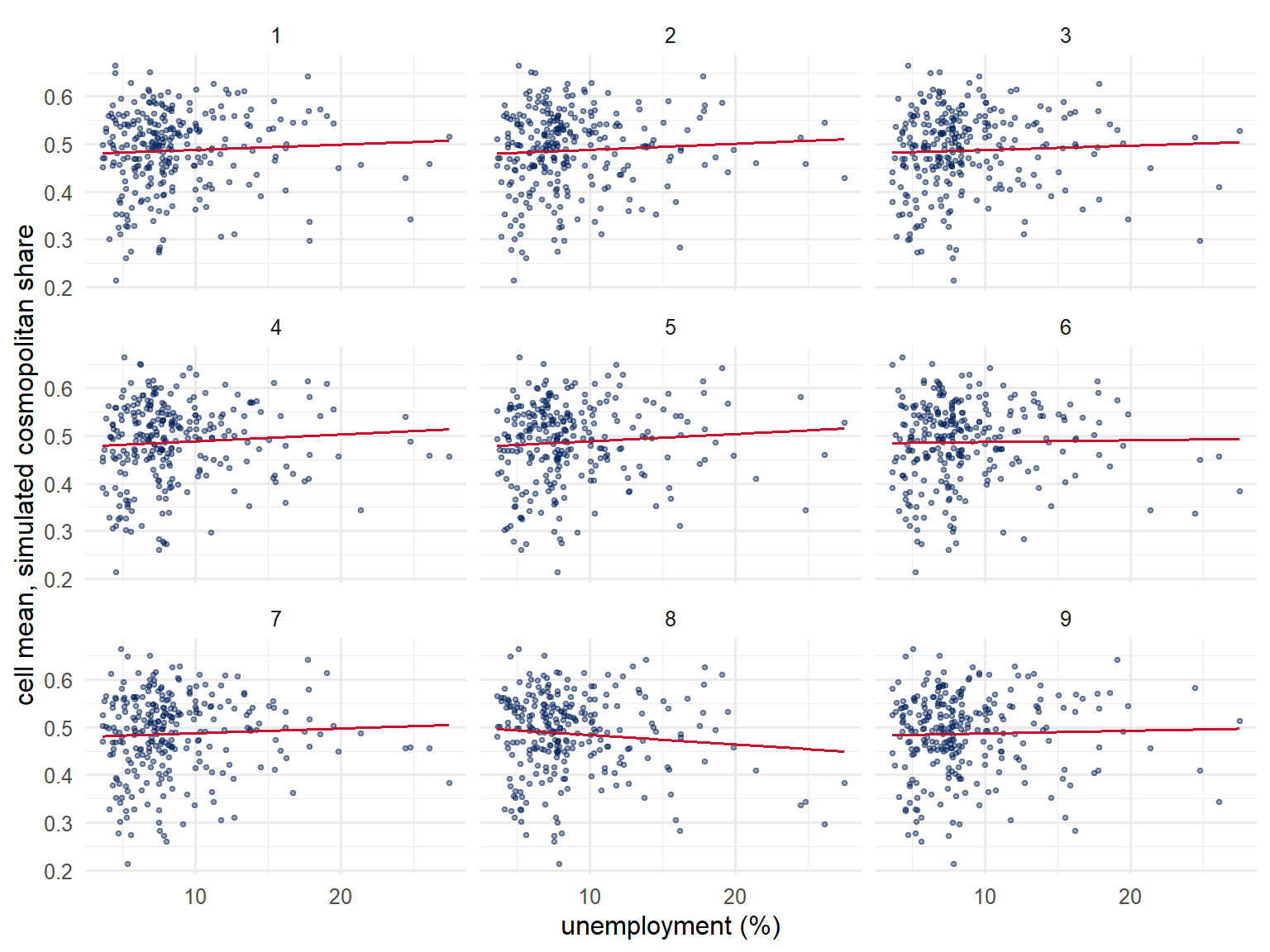
Figure 2: A lineup: nine cell-level scatters of mean simulated cosmopolitan framing against unemployment. Eight permute the unemployment series within country; one is the real structure of the twin. Pick the panel that looks like an effect before reading on.
NoteWhich panel is real?
Panel 8. If you picked it, you have informally rejected the null by eye, which is the logic of a permutation test applied visually. If you could not, that is itself evidence about how strong a level-2 relationship of this size looks at this sample size.
9. Design checks
Power analysis for multilevel designs rarely has clean formulas, and the standard advice is to simulate: generate data from the design you are contemplating and see how precisely it estimates the quantity you care about (Gelman et al. 2020; DeBruine and Barr 2021). Precision on a level-2 slope, the slope of a predictor measured for countries or country-years, comes mainly from the number of countries and years and much less from the number of respondents, so the useful comparison is what four times as many of each would give.
# A tibble: 3 × 4
  countries respondents       se    df
      <dbl>       <dbl>    <dbl> <dbl>
1        27       41700 0.000895   256
2        27      167000 0.000757   253
3       108      167000 0.000409  1060
Quadrupling the respondents inside the existing country-years does improve precision, but much less than quadrupling the countries does, and it adds almost no degrees of freedom, because the number of units that provide independent information about unemployment has not changed. No feasible amount of extra survey data inside the existing 27 countries would do what 81 more countries would, and no choice on the specification menu can manufacture level-2 information that the design does not contain. That is why the estimates in this literature have wide uncertainty bands, and simulation can measure the best precision that a design could reach before any data are collected under it. A methodological literature sets out how to do this systematically, by stating the aims, data-generating mechanisms, estimands, methods and performance measures of a simulation study before it is run (Morris et al. 2019), and it is the natural next reading.
Further reading
Four things to read next. For the habit itself, Regression and Other Stories is the core text, with short fake-data simulations that recur throughout and build on one another (Gelman et al. 2020), and Active Statistics packages the same moves as classroom activities (Gelman and Vehtari 2024). For multilevel structures specifically, DeBruine and Barr’s tutorial covers the ground of sections 2 and 6 of this module in more depth: it builds a mixed-effects simulation from nothing and recovers its parameters, on the argument that constructing the data is how you come to understand the model (DeBruine and Barr 2021). For simulation inside a modelling workflow – prior and posterior predictive checking, calibration, experimentation on synthetic data before touching the real thing – the Bayesian workflow book is the current statement (Gelman et al. 2026), and its habits transfer well beyond Bayesian settings. And for simulation as a research method in its own right, the design framework of Morris et al. (2019) supplies the vocabulary, the book-length treatment written for social scientists is Carsey and Harden (2014), and an applied Monte Carlo study that this site already cites, on cross-lagged panel models, shows the method applied to a question close to the choice of estimator in this case (Leszczensky and Wolbring 2022).
Simulation studies are analyses too, and they have researcher degrees of freedom of their own – conditions, performance measures, which results get reported – so a comparative study can be tuned until any method looks superior (Pawel et al. 2024). The disciplines that this course keeps returning to, preregistered designs and justified choices, apply to simulated data as much as to real data. The generator, the calibration script, the codebook and the code chunks on this page are all committed, so the first Try-it is the quickest place to begin: change what the recipe plants, rerun, and watch what your tools do when you already know the answer.
References
Carsey, Thomas M., and Jeffrey J. Harden. 2014. Monte Carlo Simulation and Resampling Methods for Social Science. SAGE Publications. https://doi.org/10.4135/9781483319605.
DeBruine, Lisa M., and Dale J. Barr. 2021. “Understanding Mixed-Effects Models Through Data Simulation.”Advances in Methods and Practices in Psychological Science 4 (1): 2515245920965119. https://doi.org/10.1177/2515245920965119.
Gelman, Andrew, Jennifer Hill, and Aki Vehtari. 2020. Regression and Other Stories. Cambridge University Press. https://doi.org/10.1017/9781139161879.
Gelman, Andrew, and Aki Vehtari. 2024. Active Statistics: Stories, Games, Problems, and Hands-on Demonstrations for Applied Regression and Causal Inference. Cambridge University Press.
Gelman, Andrew, Aki Vehtari, Richard McElreath, et al. 2026. Bayesian Workflow. First edition. CRC Press.
Leszczensky, Lars, and Tobias Wolbring. 2022. “How to Deal with Reverse Causality Using Panel Data? Recommendations for Researchers Based on a Simulation Study.”Sociological Methods & Research 51 (2): 837–65. https://doi.org/10.1177/0049124119882473.
Morris, Tim P., Ian R. White, and Michael J. Crowther. 2019. “Using Simulation Studies to Evaluate Statistical Methods.”Statistics in Medicine 38 (11): 2074–102. https://doi.org/10.1002/sim.8086.
Pawel, Samuel, Lucas Kook, and Kelly Reeve. 2024. “Pitfalls and Potentials in Simulation Studies: Questionable Research Practices in Comparative Simulation Studies Allow for Spurious Claims of Superiority of Any Method.”Biometrical Journal 66 (1): e2200091. https://doi.org/10.1002/bimj.202200091.