| No-opinion rule | Specifications | Claim direction | Significant | Median aligned r |
|---|---|---|---|---|
| zero | 144,768 | 68.8% | 57.2% | −0.121 |
| drop | 144,768 | 69.4% | 58.4% | −0.129 |
| split | 144,768 | 69.2% | 58.4% | −0.128 |
| imputed (mice) | 1,560 | 66.2% | 61.3% | −0.171 |
| imputed (Amelia) | 1,560 | 66.0% | 61.4% | −0.176 |
Missing answers
The respondents who mentioned nothing, and the conventions for them
The specification menu has an axis called no-opinion handling with five settings, and this module explains why it is there. Of the 416,698 respondents in the EU-frames data, 26,325 (6.3%) answered the question “What does the EU mean to you personally?” by mentioning none of the thirteen things on the list, so that on every framing scale their score is zero divided by zero. The original paper and its five reanalyses resolved that in two different ways without saying so, and the people concerned are not a random slice of the sample.
The missing answers
The framing scales are built from a multiple-mention battery: a respondent ticks any of thirteen items, and the cosmopolitan scale is the share of their ticks that fall on the five cosmopolitan items. A respondent who ticks nothing has no share. The survey records two further codes for that person, “other (spontaneous)” and “don’t know”, and the 26,325 split three ways: 13,736 said they did not know, 3,642 gave an answer that was not on the list, and 8,947 have no tick of any kind. These are three different kinds of respondent. Someone who says the EU means something that the list did not anticipate has an opinion. Someone who says they do not know may have none, or may have one they would rather not state. A blank row may be a refusal, an interviewer’s omission or a coding gap, and the file does not say which.
The Stata code written by the original author (OA) divides the number of mentions in each framing cluster by the total number of mentions and has no rule for a zero total. Stata returns a missing value for 0/0, and the mixed model drops a missing outcome, so those respondents left her analysis without a line of code saying so. The level-1 N of 390,373 that she reported, the number of respondents in her model, is exactly the number who mentioned at least one item. The Multi100 reanalysis that produced the recorded t of −3.804 coded the same respondents 0 on every scale, and the course panel inherits that convention. One analyst, PRL47, built both versions and reported the zero one. So the published coefficient and its best-known reanalysis differ in what they assume about 6.3% of the sample, and neither states the assumption.
Whether that matters depends on who the silent respondents are. They are older, more often women, and they live in country-years with higher unemployment. Across the 270 cells the no-opinion rate correlates at 0.24 with the unemployment rate and at −0.25 with the cosmopolitan scale. The rate also differs sharply between countries: it runs at 16.0% in ES and 14.9% in GB against 1.9% in CY. Scoring the silent as zero therefore pulls the framing scale down most where unemployment is highest, which is the direction that the claim predicts, so part of the association is produced by the coding rule.
The three missingness mechanisms
The vocabulary for thinking about this comes from Rubin (1976) and is set out accessibly by Dong and Peng (2013). Data are missing completely at random when the probability that a value is missing depends on nothing in the data at all, so the observed cases are a random sample of the complete ones; dropping them costs precision and nothing else. Data are missing at random when that probability depends on things that were observed but not, once those are accounted for, on the missing value itself. In the example that Dong and Peng use, whether a post-test score is missing is a coin toss among students who scored alike on the pre-test. Data are missing not at random when the probability depends on the missing value even after the observed data are allowed for, as when high earners are the ones who decline to state their income. The labels describe the mechanism that produced the gaps, not their size, and the practical consequence is asymmetric: the first two can be handled with methods that use only the observed data, while the third requires the analyst to say how the missing values differ from the observed ones, which the data cannot reveal.
Mapped onto the case, the silent respondents are plainly not missing completely at random, since their age, sex and location predict their silence. Missing at random given age, sex, education and the country-year cell is the working assumption that every imputation below rests on. It is not testable from the observed data alone, a point that Dong and Peng (2013) make against the habit of reading a t-test on observed covariates as a test of it. What can be done is to make it more plausible by conditioning on everything that predicts silence, and then to ask how far the conclusion moves if it is wrong. That last step is the sensitivity band at the end of this module. A “don’t know” about what the EU means is a fair candidate for missing not at random, because the people least engaged with the EU are the people least likely to have a framing of it, and disengagement is not in the data.
Three levels
Item non-response on the outcome battery is the case that this module works through, but the same structure recurs at two other levels of this analysis, and the weighting module covers the first of them, unit non-response. Inside a country, some people are harder to reach or more likely to refuse the whole interview, which is unit non-response, and the Eurobarometer W1 design weight is the standard correction for the imbalance it leaves. Above the country, one reanalyst’s Eurostat table had no United Kingdom row and nothing before 2009 for any country but France and Sweden, so half the country-year cells were missing from that analysis before a single respondent was considered. Non-response rates on their own predict little about the bias that results (Groves 2006; Groves and Peytcheva 2008; Hendra and Hill 2018); what matters is whether the missing units differ from the observed ones on the quantity of interest, which is the same question at every level.
The conventions
The menu has three deterministic rules, which code every silent respondent in the same way without fitting a model, and each is a statement about what the silent respondents mean. Zero treats them as people with no framing of any kind, which is the convention of most of the reanalyses. Drop treats them as people who did not answer the question, which is what OA’s code did. Split takes the three codes at their word: “don’t know” and blank are dropped as non-response, and “other” is kept at zero on the reasoning that an answer off the list is still an answer that contains no cosmopolitan content. The rules change the cell means before any model is fitted, and the average cosmopolitan cell mean is 0.507 under zero and 0.540 under drop.
The rules also change the question. Under zero the estimand is the average framing among everyone interviewed, with silence counted as no framing; under drop it is the average framing among people who have a framing at all. Those are different populations, so by the test that is applied in the specification menu the no-opinion rule is an estimand decision. It is classed with measurement on the menu because that is where the decision is made in practice, at the moment the outcome column is built, and a participant who meets it there should know that it also changes the estimand.
Across the whole grid, the rule moves by a few points both the share of specifications that point in the direction of the claim and the share that are significant, and it moves the median correlation by a few hundredths:
: The no-opinion rule across every specification in which it varies. The two imputation rows are fitted at the standard measurement settings only. {#tbl-noop-levels}
For the published specification, the coefficient on unemployment for cosmopolitan framing, with two-way fixed effects on all 270 cells, takes the following values under the five rules:
| Rule | b | t | df | p | aligned r |
|---|---|---|---|---|---|
| zero (Multi100) | −0.00347 | −3.80 | 233 | 0.00018 | −0.242 |
| zero (Multi100) | −0.014 | −4.08 | 232 | 6.3e−05 | −0.258 |
| drop (original paper) | −0.00466 | −5.01 | 233 | 1.1e−06 | −0.312 |
| split | −0.00457 | −4.94 | 233 | 1.5e−06 | −0.308 |
| imputed, mice | −0.0041 | −4.69 | 228 | 4.7e−06 | −0.297 |
| imputed, Amelia | −0.00412 | −4.73 | 228 | 4e−06 | −0.299 |
: The published Multi100 specification of analyst C6HJR under each treatment of the respondents who mentioned nothing. {#tbl-noop-spec}
Multiple imputation
Imputation replaces a rule with a model. Instead of deciding what the silent would have said, it estimates a distribution for each missing score from the respondent’s observed characteristics and draws from it, several times over, so that the uncertainty of the guess is included in the final standard error. Dong and Peng (2013) describe the three steps: fill the gaps m times to produce m complete datasets, analyse each with the model you would have run anyway, and combine the m results with the rules that Rubin (1987) gave, under which the pooled estimate is the mean of the m estimates and its variance is the mean within-imputation variance plus the between-imputation variance inflated by a factor of 1 + 1/m. The between-imputation part expresses the uncertainty about the imputed values, and a single imputation, which sets it to zero, understates every standard error computed from it. How many imputations are enough depends on how much information is missing; Graham et al. (2007) show that the once-standard three to five are too few when the fraction of missing information is not small, and the course uses ten. The imputation model should include every variable in the analysis model and anything else that predicts either the missing values or their missingness (Collins et al. 2001; Schafer and Graham 2002), and it should not be less general than the analysis model, a condition that Meng (1994) named ‘congeniality’, and one that is easy to violate here, since the imputation happens at respondent level and the analysis at cell level.
Two engines are run on the case, because they come from different traditions and the course should show both. mice (Buuren and Groothuis-Oudshoorn 2011) imputes one variable at a time conditional on the others, cycling until the imputations settle, and the version used here draws each missing share from respondents with similar predicted values (predictive mean matching), which keeps every imputed score inside the range that a bounded scale can take (White et al. 2010). Amelia (Honaker et al. 2011; King et al. 2001) fits one multivariate normal model to all the variables at once by expectation maximisation (an iterative algorithm for fitting a model to incomplete data) with bootstrapping, the approach that was developed by Gary King and colleagues for time-series cross-section data of this shape (Honaker and King 2010). Amelia imputes by drawing from that model, and the imputed values can fall outside the unit interval and are then clipped. Both condition on age, sex, education and the country and year of interview. Each of the ten completed respondent files is aggregated to country-year means and every one of the 780 estimand cells that have unemployment as the predictor and the answers scored as shares is fitted on each, at the standard measurement settings, then pooled.
| Engine | b | t | df | Fraction of missing information |
|---|---|---|---|---|
| mice, predictive mean matching | −0.0041 | −4.69 | 228 | 0.014 |
| Amelia, EM with bootstrapping | −0.00412 | −4.73 | 228 | 0.012 |
: The published specification under multiple imputation, pooled over ten imputations by Rubin’s rules. The fraction of missing information is the share of the uncertainty about the coefficient that is due to the silent respondents. {#tbl-mi}
The two engines give estimates close to one another and close to the drop rule, which is what should happen when the imputation model conditions on the same things that distinguish the silent from the rest: under missing at random, filling the gaps from people who look like them is a more careful version of leaving them out. The gap between the imputed rows and the zero row is the part of the published result that the zero convention supplied. That is a result about this case; Lall (2016) reanalysed thirty studies in comparative and international political economy with multiple imputation in place of listwise deletion and found that the main results of fourteen of them disappeared, because in that literature the missing cases were the poorer and less democratic countries and the analyses had been run, by default, on the rest.
“Don’t know” as an answer
Survey methodologists have argued for fifty years about whether a “don’t know” is missing data or a response. Francis and Busch (1975) reviewed the early evidence; Krosnick et al. (2001) showed experimentally that offering an explicit no-opinion option does not, in general, improve the quality of the answers that remain, because many who take it could have answered; and Luskin and Bullock (2011) found the reverse for factual knowledge, where “don’t know” mostly does mean not knowing. Kuha et al. (2018) distinguish three ways of asking (encouraging a “don’t know”, accepting one neutrally, and probing it with a follow-up) and show on European Social Survey data that probing halves the rate but changes the measurement properties of the answers it extracts, so that the survey has traded an error of omission for an error of commission. The ESS itself does not probe. Who says “don’t know” is not random either: Laurison (2015) finds the willingness to state an opinion patterned by class and education, which makes non-response on attitude items a form of inequality in whose views reach the data.
That literature has two implications for this case. It supports treating a “don’t know” about the EU as non-response rather than as zero framing, which is the split rule and the imputation option. It also warns that a group defined by not answering cannot be assumed to resemble the group that did, so the missing-at-random assumption behind imputation is where a critic would press. The “other” code in the battery is more reassuring, since 3,642 people volunteered a meaning that the list did not offer, and each of those answers is an opinion.
Sensitivity to the assumption
Nothing in the observed data can distinguish missing at random from missing not at random; Molenberghs et al. (2008) prove that for any model of the latter there is a model of the former that fits the observed data equally well. The response is to show how far the conclusion depends on the assumption, and the device used here is a sensitivity band. Suppose every silent respondent would have scored what the answering respondents in their cell scored, plus some amount δ that is the same for all of them. Then each cell mean is the answered mean plus δ times the share of the cell that was silent, and the published specification can be refitted for any δ. Two values are already familiar: δ = 0 is the drop rule, and δ equal to minus the answered mean, about −0.53 here, is the zero rule.
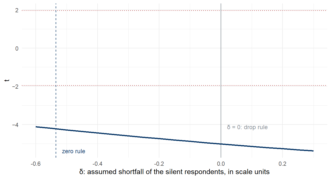
On the band, the zero convention corresponds to the assumption that everyone who stayed silent would have scored the lowest value that the scale allows. That is the most extreme missing-not-at-random assumption available, and the one that moves the result furthest in the direction of the claim. Whether any conclusion changes across the band can be read off the figure, and that is what should be reported alongside a result on these data. Reporting the missing-data treatment, the assumption it makes and the sensitivity of the result to that assumption is what Lee et al. (2021) and Sterne et al. (2009) ask for in observational research, and the proportion of missing data is not, on its own, the thing to report (Madley-Dowd et al. 2019).
What to take away
- A respondent who mentioned nothing belongs to one of three groups, and the survey codes record which. Look for the codes before choosing a rule.
- The original paper and its best-known reanalysis differ in this rule and neither states it; the coefficient recorded for analyst C6HJR in Multi100 rests on the convention that the silent have zero framing.
- Zero, drop and split are not robustness variants of one estimate. They change whose framing the average describes.
- Imputation replaces a rule with a model and includes the uncertainty of the imputed values in the result; it assumes missingness at random given what it conditions on, and that assumption is where a critic will press.
- Show the band. A result that holds across the range of defensible assumptions about the silent is a different kind of result from one that depends on the zero convention.
Exercise
- From
teney_panel_weights.csv, plot the no-opinion rate against the unemployment rate across the 270 cells and describe the pattern in one sentence. Which mechanism does it rule out? - Look up, in
data/grid/, the shard for your preregistered estimand cell (each shard contains the grid rows for one estimand cell) and compare its five no-opinion rows. Which rule is the zero rule closest to, and which furthest from? - Rewrite the estimand statement for the zero rule and for the drop rule. Which word changes?
References
Buuren, Stef van, and Karin Groothuis-Oudshoorn. 2011. “<B>mice</b>: Multivariate Imputation by Chained Equations in<i>r</i>.” Journal of Statistical Software 45 (3). https://doi.org/10.18637/jss.v045.i03.
Collins, L. M., J. L. Schafer, and C. M. Kam. 2001. “A Comparison of Inclusive and Restrictive Strategies in Modern Missing Data Procedures.” Psychological Methods 6: 330–51.
Dong, Yiran, and Chao-Ying Joanne Peng. 2013. “Principled Missing Data Methods for Researchers.” SpringerPlus 2 (1). https://doi.org/10.1186/2193-1801-2-222.
Francis, Joe D., and Lawrence Busch. 1975. “What We Now Know about ‘i Don’t Knows’.” Public Opinion Quarterly 39 (2): 207. https://doi.org/10.1086/268217.
Graham, John W., Allison E. Olchowski, and Tamika D. Gilreath. 2007. “How Many Imputations Are Really Needed? Some Practical Clarifications of Multiple Imputation Theory.” Prevention Science 8 (3): 206–13. https://doi.org/10.1007/s11121-007-0070-9.
Groves, R. M., and E. Peytcheva. 2008. “The Impact of Nonresponse Rates on Nonresponse Bias: A Meta-Analysis.” Public Opinion Quarterly 72 (2): 167–89. https://doi.org/10.1093/poq/nfn011.
Groves, Robert M. 2006. “Nonresponse Rates and Nonresponse Bias in Household Surveys.” Public Opinion Quarterly 70 (5): 646–75. https://doi.org/10.1093/poq/nfl033.
Hendra, Richard, and Aaron Hill. 2018. “Rethinking Response Rates: New Evidence of Little Relationship Between Survey Response Rates and Nonresponse Bias.” Evaluation Review 43 (5): 307–30. https://doi.org/10.1177/0193841x18807719.
Honaker, J., and G. King. 2010. “What to Do about Missing Values in Time-Series Cross-Section Data.” American Journal of Political Science 54 (2): 561–81. https://doi.org/DOI 10.1111/j.1540-5907.2010.00447.x.
Honaker, J., G. King, and M. Blackwell. 2011. “Amelia II: A Program for Missing Data.” Journal of Statistical Software 45 (7): 1–47.
King, Gary, James Honaker, Anne Joseph, and Kenneth Scheve. 2001. “Analyzing Incomplete Political Science Data: An Alternative Algorithm for Multiple Imputation.” American Political Science Review 95 (1): 49–69. https://doi.org/10.1017/S0003055401000235.
Krosnick, Jon A., Allyson L. Holbrook, Matthew K. Berent, et al. 2001. “The Impact of ‘No Opinion’ Response Options on Data Quality.” Public Opinion Quarterly 66 (3): 371–403. https://doi.org/10.1086/341394.
Kuha, Jouni, Sarah Butt, Myrsini Katsikatsou, and Chris J. Skinner. 2018. “The Effect of Probing ‘Don’t Know’ Responses on Measurement Quality and Nonresponse in Surveys.” Journal of the American Statistical Association 113 (521): 26–40. https://doi.org/10.1080/01621459.2017.1323640.
Lall, Ranjit. 2016. “How Multiple Imputation Makes a Difference.” Political Analysis 24 (4): 414–33. https://doi.org/10.1093/pan/mpw020.
Laurison, Daniel. 2015. “The Willingness to State an Opinion: Inequality, Don’t Know Responses, and Political Participation.” Sociological Forum 30 (4): 925–48. https://www.jstor.org/stable/24878707.
Lee, Katherine J., Kate M. Tilling, Rosie P. Cornish, et al. 2021. “Framework for the Treatment and Reporting of Missing Data in Observational Studies: The Treatment and Reporting of Missing Data in Observational Studies Framework.” Journal of Clinical Epidemiology 134: 79–88. https://doi.org/10.1016/j.jclinepi.2021.01.008.
Luskin, Robert C., and John G. Bullock. 2011. “‘Don’t Know’ Means ‘Don’t Know’: DK Responses and the Public’s Level of Political Knowledge.” The Journal of Politics 73 (2): 547–57. https://doi.org/10.1017/s0022381611000132.
Madley-Dowd, Paul, Rachael Hughes, Kate Tilling, and Jon Heron. 2019. “The Proportion of Missing Data Should Not Be Used to Guide Decisions on Multiple Imputation.” Journal of Clinical Epidemiology 110: 63–73. https://doi.org/10.1016/j.jclinepi.2019.02.016.
Meng, Xiao-Li. 1994. “Multiple-Imputation Inferences with Uncongenial Sources of Input.” Statistical Science 9 (4). https://doi.org/10.1214/ss/1177010269.
Molenberghs, Geert, Caroline Beunckens, Cristina Sotto, and Michael G. Kenward. 2008. “Every Missingness Not at Random Model Has a Missingness at Random Counterpart with Equal Fit.” Journal of the Royal Statistical Society Series B: Statistical Methodology 70 (2): 371–88. https://doi.org/10.1111/j.1467-9868.2007.00640.x.
Rubin, Donald B. 1976. “Inference and Missing Data.” Biometrika 63 (3): 581–92. https://doi.org/10.2307/2335739.
Rubin, Donald B. 1987. Multiple Imputation for Nonresponse in Surveys. In Wiley Series in Probability and Statistics. Wiley. https://doi.org/10.1002/9780470316696.
Schafer, Joseph L., and John W. Graham. 2002. “Missing Data: Our View of the State of the Art.” Psychological Methods 7 (2): 147–77. https://doi.org/10.1037/1082-989x.7.2.147.
Sterne, J. A C, I. R White, J. B Carlin, et al. 2009. “Multiple Imputation for Missing Data in Epidemiological and Clinical Research: Potential and Pitfalls.” BMJ 338 (jun29 1): b2393–93. https://doi.org/10.1136/bmj.b2393.
White, Ian R., Patrick Royston, and Angela M. Wood. 2010. “Multiple Imputation Using Chained Equations: Issues and Guidance for Practice.” Statistics in Medicine 30 (4): 377–99. https://doi.org/10.1002/sim.4067.