The items behind the scales

The Eurobarometer question, the four published scales and the two composites, item by item

Every outcome on the specification menu is built from one survey question, and the six scales that the menu offers as its frame set are six ways of adding up the answers to it. The menu treats the choice among them as a decision about what the claim is about, and the choice of scoring rule, a share of a respondent’s own mentions or a count of the items in the set, as a second decision of the same kind. It does not, however, show the instrument itself. This module takes the thirteen answer options apart: how often each is named, how the answers to them hang together, how many dimensions they hold, whether those dimensions are the four that the original author (OA) built and the course inherits, and how far a scale of two items can be trusted as a measure. The subject is measurement rather than modelling. Nothing here changes which scales the course uses, for reasons that are given in the closing section, but the page should leave you knowing more about the numbers before you choose one.

The tables on this page are read from files that were written before the page was built. The respondent-level records are GESIS-licensed and are not distributed with the course, so the analyses were run once, on the facilitator’s machine, by companion/_model-outputs/fit_measurement.R, and only aggregate tables were committed: item prevalences, a correlation matrix, eigenvalues, loadings and fit indices. The correlation matrix is enough to repeat every exploratory step below without the microdata, and the Try it section at the end does so.

1. The instrument

The question is the Eurobarometer item that asks “What does the European Union mean to you personally?”, with a card of fourteen answers of which any number may be chosen, and it is the source of every framing scale in the case. OA sets one of the fourteen aside, the Euro, and builds the four scales from the remaining thirteen (Teney 2016, 623), grounding the grouping in an earlier categorical principal component analysis of a single wave which had found that “these answer categories build four distinct dimensions of EU framing across the 27 EU countries” (Teney 2016, 623). The construction of each scale is stated in one sentence: “For each of the framing dimensions, the scale is composed of the sum of the mentioned items belonging to the specific framing dimension, divided by the total number of items mentioned by the respondent”, so that the four scales “measure the relative frequency with which the respondent associates each frame to the EU” (Teney 2016, 623). That sentence is the share rule of the menu, and the count rule and the per-item rate are the two departures from it that the Multi100 analysts and the course have taken.

Table 1 lists the thirteen answers under the scale each was assigned to, with the share of all 416,698 respondents who named it. The course adds two composites to the four published scales, a positive one made of the cosmopolitan and utilitarian items together and a negative one made of the communitarian and libertarian items together, because the claim under test speaks of positive and negative dimensions in the plural and singles out none of them.

prev |>
  mutate(scale = factor(scale, scale_order), valence = if_else(valence == "positive", "positive", "negative")) |>
  arrange(scale) |>
  transmute(Item = item, Scale = as.character(scale), Valence = valence, `Named by` = pct(share_mentioning)) |>
  tt() |>
  style_tt(j = 4, align = "r")

Table 1: The thirteen answer options, the scale each was assigned to in the original paper, and the share of respondents naming each. The ‘Euro’ option is the fourteenth and is set aside throughout, following the original paper. Shares are over all respondents interviewed in the sixteen waves, those who named nothing included.

Item	Scale	Valence	Named by
Peace	cosmopolitan	positive	28.5%
Democracy	cosmopolitan	positive	21.9%
Freedom to travel	cosmopolitan	positive	51.0%
Cultural diversity	cosmopolitan	positive	22.1%
Stronger say in the world	cosmopolitan	positive	23.1%
Economic prosperity	utilitarian	positive	18.7%
Social protection	utilitarian	positive	11.9%
Unemployment	communitarian	negative	16.6%
Loss of cultural identity	communitarian	negative	12.1%
More crime	communitarian	negative	17.5%
Not enough border control	communitarian	negative	16.6%
Bureaucracy	libertarian	negative	21.5%
Waste of money	libertarian	negative	21.6%

Freedom to travel is the one answer that about half of respondents give, and the rest are named by between roughly a tenth and three tenths, with social protection and the loss of cultural identity the rarest. Those prevalences matter for what follows, because a scale is only as informative as the answers it is made of, and a scale of two rarely named items has less to work with than a scale of five common ones.

2. The theory behind the grouping

The four published scales are a theory, stated before any correlation was computed, and the paper sets it out in one sentence: the items “can be clustered into four distinct EU-framing dimensions endorsed by European citizens: two positive and two negative; two referring to a materialist and two related to a non-materialist understanding of the EU” (Teney 2016, 620). Two axes cross. Valence separates the answers that praise the Union from the answers that blame it. Materialism separates the answers about money and welfare from the answers about peace, democracy, identity and borders. Each scale is one cell of the resulting two-by-two. The utilitarian scale is “the positive materialist dimension”, the libertarian scale “the negative materialist dimension”, the cosmopolitan scale “the positive non-materialist dimension” and the communitarian scale “the negative non-materialist dimension” (Teney 2016, 620).

The paper relies on that design again in its hypotheses, which is why it is worth examining here. The first hypothesis has two sentences, and only the first of them appears on the Multi100 claim card: “Poor national economic performances significantly increase the negative and decrease the positive EU-framing dimensions. The effect is stronger on the materialist dimensions of EU framing” (Teney 2016, 621). The second sentence compares cells of the two-by-two with one another, and the comparison presupposes that the two materialist scales and the two non-materialist scales are what the theory says they are. The second hypothesis, about the education gap, makes the same presupposition when it predicts that poor economic performance narrows the gap more on the materialist dimensions.

The sections that follow put to the data the question that the theory answered in advance: how do the thirteen answers hang together, and how many dimensions do they hold? The valence axis will come through clearly. The materialist axis will come through on one side of the valence line and not on the other, and section 8 says what that leaves of the two sentences above. Neither kind of grouping is wrong in itself. A scale defined by theory can be compared with published work and with other analysts, which is what a replication needs, while a scale defined by the data fits the data from which it was cut. The two groupings can disagree, and here they partly do, so the grouping on which a claim is tested is a decision that the analyst makes, whether or not the decision is stated.

3. The correlations among the items

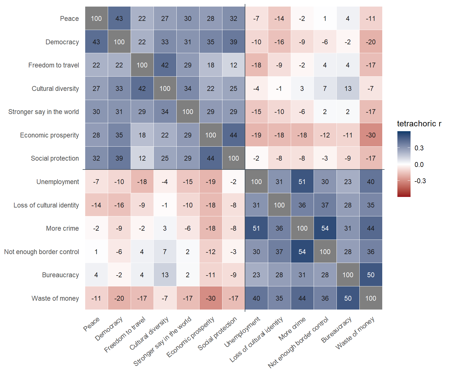
Each answer is a yes or a no, and the ordinary correlation between two yes-or-no variables is bounded below one by their marginal frequencies whenever those frequencies differ, so that an item named by a quarter of respondents and an item named by half can never correlate at more than about 0.58 however closely they go together. The usual remedy in measurement work is the tetrachoric correlation, which treats each binary answer as the visible part of an underlying continuous propensity to give it and estimates the correlation between the two propensities. It is the correlation that factor analysis of binary items is built on, and Figure 1 shows all seventy-eight of them, arranged with the two positive scales first and the two negative ones after.

tet_plot <- tet |>
  mutate(item = factor(item, item_order), with = factor(with, rev(item_order)))
ggplot(tet_plot, aes(item, with, fill = tetrachoric)) +
  geom_tile(colour = "white") +
  geom_text(aes(label = round(100 * tetrachoric)), size = 3,
            colour = ifelse(abs(tet_plot$tetrachoric) > 0.45, "white", "#1a1a1a")) +
  scale_fill_gradient2(low = "#96131b", mid = "white", high = "#0e3b6a", limits = c(-0.6, 0.6),
                       name = "tetrachoric r") +
  geom_hline(yintercept = 13 - 7 + 0.5, colour = "#3c4a56") +
  geom_vline(xintercept = 7.5, colour = "#3c4a56") +
  labs(x = NULL, y = NULL) +
  theme_minimal(base_size = 11) +
  theme(axis.text.x = element_text(angle = 40, hjust = 1), panel.grid = element_blank(),
        legend.position = "right")

Figure 1: Tetrachoric correlations among the thirteen items, times one hundred, over all respondents. Items are ordered by the scale they were assigned to: cosmopolitan and utilitarian above the line, communitarian and libertarian below it.

The items divide first by valence. The seven positive items correlate positively with one another, at between roughly 0.12 and 0.44, the six negative items likewise at between 0.23 and 0.54, and the correlations across the line are close to zero or mildly negative, the strongest of them being the −0.30 between economic prosperity and waste of money. The original paper reports the same shape at the level of the four scales, with “the two positive EU framing and … the two negative EU-framing dimensions” associated at 0.27 and 0.26 and the associations across the valence line “low” (Teney 2016, 625). The item-level matrix also shows where the structure within each valence lies. On the negative side the two libertarian items, bureaucracy and waste of money, correlate at 0.50 with each other and more weakly with the communitarian four, while more crime and border control correlate at 0.54. On the positive side the strongest pairs, social protection with economic prosperity at 0.44, peace with democracy at 0.43 and freedom to travel with cultural diversity at 0.42, each lie within a published scale, but democracy correlates with social protection at 0.39 and with freedom to travel at only 0.22, so that the utilitarian pair are more closely related to peace and democracy than are freedom to travel and cultural diversity, the two mobility items of the cosmopolitan scale to which peace and democracy also belong. That is the first sign of what the factor analysis below makes explicit.

The unemployment item, which the original paper counts among the communitarian meanings of the EU, bears on a decision elsewhere on the menu. It correlates at −0.19 with economic prosperity and at −0.18 with freedom to travel, and it is the item that a robustness check in the paper removes from the communitarian scale because “it could be theoretically argued that unemployment does not constitute a component of a communitarian understanding of the EU” (Teney 2016, 633, fn. 5). The menu offers that removal as its item-set decision.

4. Dimensions

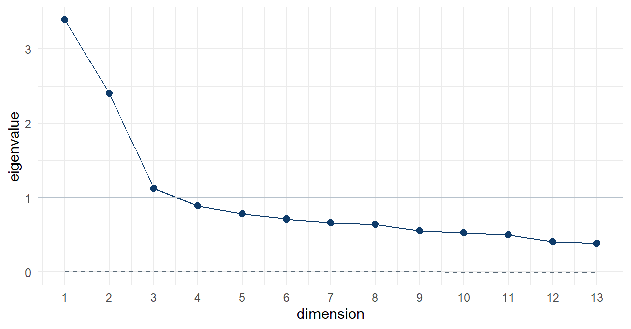
A correlation matrix of thirteen items has thirteen eigenvalues, and their sizes indicate how much of the shared variation among the items a given number of underlying dimensions would account for. Figure 2 plots them. The first two stand well clear of the rest, at 3.39 and 2.40, a third is at 1.13, and everything after it falls below one, which is the conventional line for a dimension worth keeping.

ggplot(eig, aes(factor, eigenvalue)) +
  geom_line(aes(y = parallel_mean), linetype = "dashed", colour = "#5b6b78") +
  geom_line(colour = "#0e3b6a") +
  geom_point(colour = "#0e3b6a", size = 2.2) +
  geom_hline(yintercept = 1, colour = "#b7c2cc") +
  scale_x_continuous(breaks = 1:13) +
  labs(x = "dimension", y = "eigenvalue") +
  theme_minimal(base_size = 11)

Figure 2: Eigenvalues of the tetrachoric matrix (points), with the mean eigenvalue of random data of the same size (dashed) from a parallel analysis. With over four hundred thousand respondents the random benchmark is almost exactly one, so the parallel analysis is a formality here, and what matters is the size of the gaps between the eigenvalues.

Read as a count of dimensions, the figure suggests two with a possible third, and the count rests on the items alone, without any assumption about which answers belong together. Two dimensions would be the valence split that the correlation matrix has already shown, and the next section asks whether a third and a fourth are the published split within each valence. The parallel analysis that is usually consulted at this point, which compares each eigenvalue with what random data of the same dimensions would produce, suggests five, but with 416,698 respondents the random benchmark is almost exactly one for every dimension, so that criterion reduces to counting eigenvalues above one and has little to add at this sample size.

5. Exploratory solutions

Exploratory factor analysis asks which underlying dimensions, unconstrained by any prior assignment, best reproduce the correlations among the items, and reports for each item how strongly it belongs to each dimension. The solutions below were extracted by minimum-residual factoring from the tetrachoric matrix and rotated obliquely, which allows the dimensions to correlate with one another as substantive dimensions of an attitude generally do. Table 2 gives the four-factor solution, with the assignment made in the original paper beside each item, and loadings below 0.30 blanked so that the structure can be read at a glance; the two-factor solution follows in prose.

show <- function(x) ifelse(abs(x) < 0.30, "", num(x))
l4 |>
  mutate(item = factor(item, item_order)) |>
  arrange(item) |>
  transmute(Item = as.character(item), `Published scale` = scale,
            `Factor 1` = show(F1), `Factor 2` = show(F2), `Factor 3` = show(F3), `Factor 4` = show(F4),
            Communality = num(communality)) |>
  tt() |>
  style_tt(j = 3:7, align = "r")

Table 2: The four-factor exploratory solution (minimum residual, oblimin rotation), accounting for 43.9% of the variance in the items. Loadings under 0.30 are blank. Communality is the share of the variance of an item that the four factors reproduce together. Factor correlations: 1 with 4, 0.41; 2 with 3, 0.58; every positive factor with every negative one between −0.16 and −0.02.

Item	Published scale	Factor 1	Factor 2	Factor 3	Factor 4	Communality
Peace	cosmopolitan	0.51				0.32
Democracy	cosmopolitan	0.60				0.42
Freedom to travel	cosmopolitan				0.71	0.49
Cultural diversity	cosmopolitan				0.48	0.41
Stronger say in the world	cosmopolitan	0.35			0.30	0.30
Economic prosperity	utilitarian	0.54				0.37
Social protection	utilitarian	0.72				0.47
Unemployment	communitarian		0.52			0.40
Loss of cultural identity	communitarian		0.40			0.28
More crime	communitarian		0.83			0.67
Not enough border control	communitarian		0.63			0.43
Bureaucracy	libertarian			0.75		0.53
Waste of money	libertarian			0.62		0.62

Two of the four factors reproduce the two negative scales of the original paper, item for item. The communitarian four, unemployment, loss of cultural identity, more crime and border control, load on one factor and on nothing else, with more crime the strongest at 0.83; bureaucracy and waste of money load on a factor of their own at 0.75 and 0.62. The two are distinct and related, correlating at 0.58, which is the pattern one would want from two dimensions of a single negative stance towards the EU. The positive side does not reproduce the published split. Peace, democracy, economic prosperity and social protection form one factor, cutting across the line between cosmopolitan and utilitarian framing, and it is the two utilitarian items that load highest on it; freedom to travel and cultural diversity form another, with stronger say in the world divided between the two at 0.35 and 0.30. Read substantively, the data split the positive meanings of the EU not into a civic and an economic set but into a set of benefits that the EU delivers, peace and democracy alongside prosperity and protection, and a set of things that the EU lets one do and be, travel and diversity, with a stronger say in the world belonging a little to each. The two positive factors correlate at 0.41, which is lower than the correlation between the two negative ones.

The two-factor solution is simpler still, and it is the solution to which the eigenvalues point first. Every positive item loads on one factor, at between 0.44 and 0.62, every negative item on the other, at between 0.51 and 0.75, no item loads above 0.30 on the wrong side, and the two factors correlate at −0.19. That is a clean valence structure, and it is the structure behind the two composites that the course adds: a positive scale of seven items and a negative scale of six are what the instrument most plainly measures, and each of the finer scales is a subset of one of them.

6. A confirmatory comparison

An exploratory solution is chosen by the data, so it is bound to fit the data it was chosen from. A confirmatory model states an assignment of items to dimensions in advance and asks how far the correlations it implies depart from the correlations found. Table 3 compares three such models, fitted to the binary items by diagonally weighted least squares, the estimator built for this kind of data: the published four-scale model, the four-factor model read off Table 2 with stronger say in the world allowed to belong to both positive factors, and the two-factor valence model. The indices are the usual ones. The comparative fit index and the Tucker–Lewis index read upward towards one, and the root mean square error of approximation and the standardised root mean square residual read downward towards zero. By the customary thresholds a comparative fit index above 0.95 and a root mean square error below 0.05 count as good, and the chi-square is reported for completeness only, because with 416,698 respondents it rejects every model that is not exactly true.

cfa |>
  mutate(model = c(published = "Published four scales", data_driven = "Data-driven four factors", valence = "Two valence factors")[model]) |>
  transmute(Model = model, `Chi-square (df)` = sprintf("%s (%d)", big(round(chisq)), as.integer(df)),
            CFI = num(cfi, 3), TLI = num(tli, 3), RMSEA = num(rmsea, 3), SRMR = num(srmr, 3)) |>
  tt() |>
  style_tt(j = 2:6, align = "r")

Table 3: Three confirmatory models of the thirteen items, fitted on all respondents with the diagonally weighted least squares estimator and robust corrections. The data-driven model is the four-factor exploratory structure refitted as a confirmatory one, and is expected to fit better than the published model on the data it was read from.

Model	Chi-square (df)	CFI	TLI	RMSEA	SRMR
Published four scales	42,153 (59)	0.910	0.882	0.041	0.060
Data-driven four factors	36,257 (58)	0.923	0.896	0.039	0.056
Two valence factors	57,825 (64)	0.877	0.850	0.047	0.071

The three models order as the exploratory analysis leads one to expect, and none of them reaches the conventional threshold of 0.95 on the comparative fit index. The data-driven model does best on every index, with a comparative fit index of 0.923 against 0.910 for the published scales and 0.877 for the valence model, and the root mean square error is below 0.05 for all three, at 0.039, 0.041 and 0.047. The published scales are a defensible reading of the items, though not a privileged one. A structure read off the data fits better, as it is bound to, and the difference between the two is confined to the positive side, where economic prosperity and social protection load with peace and democracy instead of forming a scale of their own. At the same time, the finer structure improves on the valence split by a margin that is real but modest, so a reader who prefers the two composites for their reliability, which the next section quantifies, or for their fit to the wording of the claim, gives up less than the four-scale vocabulary suggests.

7. Reliability

How far a short scale, such as one of two answers, can be trusted as a measure of a single disposition is a standard question in measurement, answered by a reliability coefficient. Table 4 gives, for the four published scales and the two composites, the number of items, their mean tetrachoric correlation, and the ordinal alpha that follows from the two, which is the familiar reliability coefficient computed on the tetrachoric rather than the ordinary correlations and read on the same scale, one being perfect consistency among the items.

rel |>
  mutate(scale = factor(scale, c(scale_order, "positive", "negative"))) |>
  arrange(scale) |>
  transmute(Scale = as.character(scale), Items = items, `Mean tetrachoric r` = num(mean_tetrachoric),
            `Ordinal alpha` = num(ordinal_alpha), `Mean prevalence` = pct(mean_prevalence)) |>
  tt() |>
  style_tt(j = 2:5, align = "r")

Table 4: Reliability of the six scales on the menu, from the tetrachoric correlations among their items. Ordinal alpha is Cronbach’s alpha computed on the tetrachoric matrix. Mean prevalence is the average share of respondents naming an item of the scale.

Scale	Items	Mean tetrachoric r	Ordinal alpha	Mean prevalence
cosmopolitan	5	0.31	0.69	29.3%
utilitarian	2	0.44	0.61	15.3%
communitarian	4	0.40	0.73	15.7%
libertarian	2	0.50	0.67	21.6%
positive	7	0.30	0.75	25.3%
negative	6	0.37	0.78	17.7%

The two composites are the most reliable constructs on the menu, at 0.75 and 0.78, because reliability grows with the number of items as well as with their agreement, and the two two-item scales are the least, the utilitarian at 0.61 and the libertarian at 0.67, although the two libertarian items agree with each other more closely than the items of either positive scale do. In the country-year panel on which the course fits its models, a low reliability means that the cell mean of a two-item scale is noisier for the same number of respondents, so that an association with unemployment is harder to detect on the utilitarian scale than on the cosmopolitan one, for a reason unrelated to whether the association exists. Reliability is a property of the construct, which is why the menu does not offer it as a choice. It still bears on the choice of outcome, and it is one of the reasons for the care with which the outcome axis is read on the results page.

8. Consequences for the menu

When the results are set against the theory of section 2, the valence axis is recovered in full, and the first division among the items is between praise and blame. The materialist axis is recovered on the negative side, where the communitarian and libertarian items come apart exactly as the paper assigns them, and not on the positive side, where the items divide into the benefits that the Union delivers (peace, democracy, prosperity, social protection) and the mobility and diversity it permits (freedom to travel, cultural diversity), a line that cuts across the utilitarian and cosmopolitan scales. The second sentence of the first hypothesis, “the effect is stronger on the materialist dimensions”, is thereby left as a comparison in which one of the two materialist scales is supported by the data and the other is a theoretical grouping that the data do not reproduce. The claim card that the Multi100 analysts received contained the first sentence only, so none of the five reanalyses tested the comparison. This course does not test it either, and the multiverse module and the exercise overview explain why choosing which sentence to replicate is itself the first specification decision.

The course keeps the four published scales and the two composites as the frame set, in the knowledge of what the analyses on this page show about each of them. The published scales are the vocabulary of the claim under test and of the five reanalyses, and comparability with both is worth more to a replication exercise than a structure that fits a little better on the data it was read from. The two negative scales are, in any case, recovered by the data item for item. The composites were added by the course, and they have the strongest support in the items: the valence split is the first thing the eigenvalues show, the two-factor solution is clean, and the composites are the most reliable scales on the menu. The page argues against treating the assignment of items to scales as a further fork of the multiverse. Which items make up ‘cosmopolitan framing’ is a question about the validity of a measure of a named construct, and the evidence above is the right kind of evidence for it. Which construct the claim is about is a separate matter, so a menu that offered alternative groupings as options would be asking participants to settle by choice a question that the item analyses have already addressed.

The scoring rule is a different kind of decision, one about the question itself, and the menu places it at Level 1 for that reason. Whether a respondent’s answers enter as a share of their own mentions, as a count of the items in the set, or as that count divided by the number of items in the set changes what ‘more cosmopolitan framing’ means, from the weight of a framing among the frames that a person holds to the volume of it, and no analysis of the items can settle it, because the items are the same under every rule. The specification menu offers the three rules as a decision about the question, and the per-item rate is the version that puts a two-item and a five-item scale on one footing, which after Table 4 is a consideration in its favour.

Try it

The committed correlation matrix is all that the exploratory analyses need. The code below rebuilds it from companion/_model-outputs/items_tetrachoric.csv, refits the four-factor solution of Table 2, and then asks for three factors, which is the solution that the eigenvalues leave open and which the page does not show. Where stronger say in the world goes, and which of the two positive factors survives when only one is allowed beside the two negative ones, is the question to answer.

library(dplyr); library(tidyr); library(psych)
tet <- read.csv("companion/_model-outputs/items_tetrachoric.csv") |>
  pivot_wider(names_from = with, values_from = tetrachoric)
R <- as.matrix(tet[, -1]); rownames(R) <- tet$item
n <- 416698

fa(R, nfactors = 4, n.obs = n, fm = "minres", rotate = "oblimin")   # the table above
fa(R, nfactors = 3, n.obs = n, fm = "minres", rotate = "oblimin")   # the open question

A second exercise stays closer to the menu. Fit the four-factor solution with a varimax rotation instead, which forces the factors to be uncorrelated, and compare the loadings of the two negative factors with the oblique ones above. The difference reflects the correlation of 0.58 between them.

Sources and provenance

The question wording, the assignment of items to the four scales and the share rule are taken from the original paper (Teney 2016, 623 and 625), and its removal of the unemployment item as a robustness check from its fifth footnote. Every number on this page was computed by companion/_model-outputs/fit_measurement.R on the respondent-level rebuild of the sixteen GESIS waves that the statistical methods module describes, with the tetrachoric correlations and the exploratory solutions from the psych package and the confirmatory models from lavaan, and only the aggregate tables it writes are committed: the prevalences, the tetrachoric matrix, the eigenvalues with their parallel-analysis benchmark, the loadings and factor correlations of the two exploratory solutions, the fit indices and standardised loadings of the three confirmatory models, and the reliability table. The respondent-level file is never distributed with the course, and the data sources module explains the registration route to the raw data.

References

Teney, Céline. 2016. “Does the EU Economic Crisis Undermine Subjective Europeanization? Assessing the Dynamics of Citizens’ EU Framing Between 2004 and 2013.” European Sociological Review 32 (5): 619–33. https://doi.org/10.1093/esr/jcw008.