Intermediate – one item of the battery as the outcome: logit, probit and average marginal effects
This module of the companion curriculum fits the simplest generalised linear model there is, a model for a yes-or-no outcome, on the simplest outcome in the course: one item of the question that asks what the European Union means to the respondent personally. Every framing scale on the specification menu is built from thirteen such items, so an item is the rung of the data ladder below every scale, and a model for one item is the building block under everything that the statistics module fits to the scales and that the items module says about how they hang together. The page follows two items: “Unemployment”, the answer that shares its content with the predictor of the whole case, and “Peace”, the most-named positive answer after freedom to travel.
Everything here was fitted on the real respondents, the 408,055 people in the file that the build script of the workspace produces from the sixteen GESIS surveys, and written out as the aggregate tables that the page reads; the respondent codebook describes the variables. The script that fitted them, companion/_model-outputs/fit_items_glm.R, runs on that file, so anyone who has built it can refit every model on this page. The module assumes only the R module and section 2 of the statistics module, on the first linear model.
1. A yes-or-no outcome
A respondent either named “Unemployment” as something the EU means to them or did not. The outcome is 0 or 1, and a model of it describes the probability of a 1: for a respondent of a given kind, how likely it is that unemployment is among the things the EU means to them, and how that likelihood differs between kinds of respondent and between country-years.
A linear model can be fitted to a 0/1 outcome, and often is, under the name of the linear probability model. Its coefficients are differences in probability, which is the easiest scale to read, and with a large sample and probabilities away from the edges it does little harm. It has two well-known faults. Its predicted probabilities can fall below 0 or above 1, because a straight line has no floor or ceiling; and its errors cannot have constant variance, because a 0/1 variable with probability p has variance p(1 − p), which changes with p. The generalised linear model repairs both, by modelling a transformation of the probability, one that runs over the whole real line, and by using an estimator that treats the outcome as binary. The two transformations in common use are the logit, the log of the odds p/(1 − p), and the probit, the point on a standard normal distribution below which a share p of the area lies. A coefficient in a logit model is a difference in log-odds, and a coefficient in a probit model is a difference in standard-normal units. Neither is a probability, and section 5 is about getting back to one.
2. Who names unemployment, and when
The two items differ in level and in who names them. “Peace” is named by about 29.1% of respondents across the ten years and “Unemployment” by about 16.6%, and both move with the education of the respondent, in opposite directions.
Table 1: Share of respondents naming each item, by education band. Bands are the published ones, from the age at which full-time education finished.
Item
Education
Named by
Respondents
Peace
low
26.4%
85,698
Peace
mid
26.9%
191,359
Peace
high
32.8%
130,998
Unemployment
low
22.0%
85,698
Unemployment
mid
17.7%
191,359
Unemployment
high
11.6%
130,998
The low-educated name unemployment almost twice as often as the high-educated, 22.0% against 11.6%, and the high-educated name peace more often than the low-educated, 32.8% against 26.4%. Before any model has been fitted, those two differences are the raw material of the first part of the second hypothesis of the original paper, H2a, that the high-educated frame the EU more positively and less negatively.
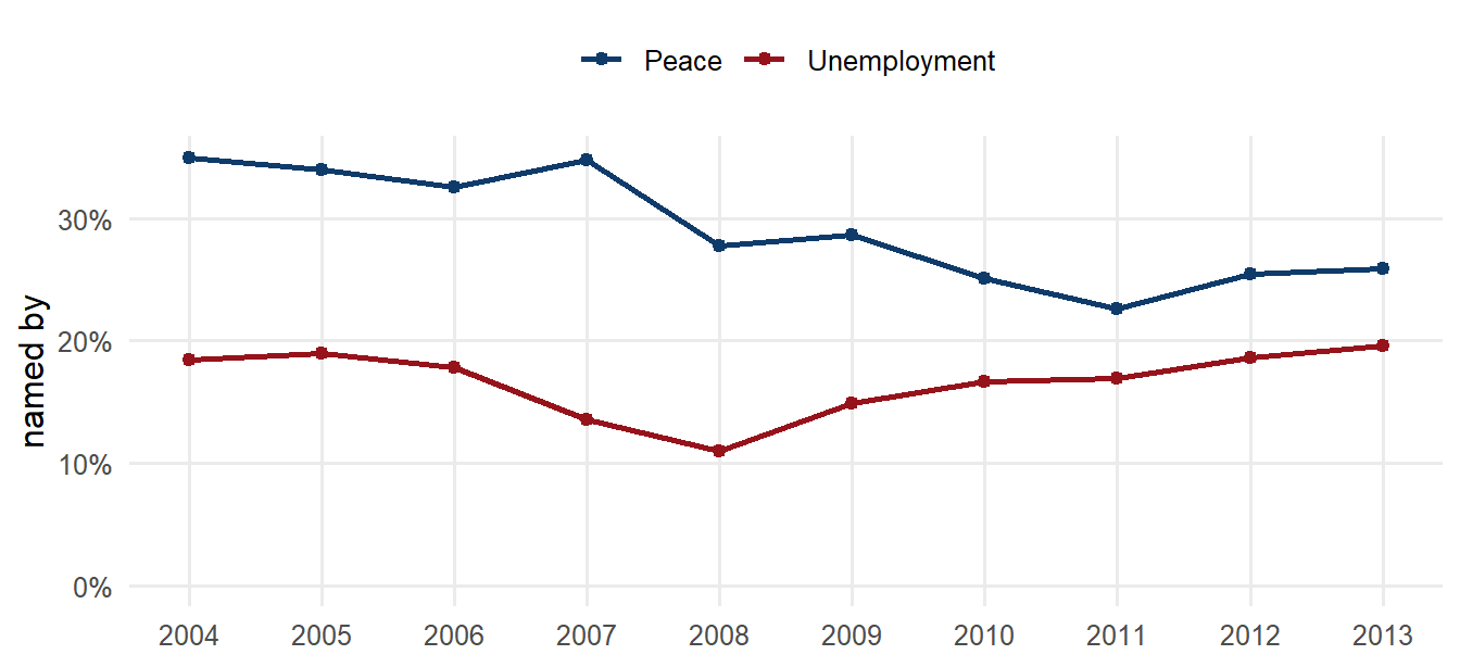
Figure 1: Share of respondents naming each item, by fieldwork year, across the twenty-seven member states.
Both items also change over the decade. “Unemployment” falls from 18.5% in 2004 to 10.9% in 2008, the last year before the crisis reached the labour market, and climbs back to 19.6% by 2013. “Peace” declines from 34.9% to 22.6% in 2011. That the item which names the predictor of the case tracks the predictor so visibly is one reason that the specification menu offers an item set without it.
3. Logit and probit, side by side
Both links are fitted with the same predictors: the three education bands, age, sex, the eight occupational groups and the three types of community, which is the respondent-level part of the published models. The coefficients are on different scales and the table shows them next to each other.
Table 2: Logit and probit coefficients for naming ‘Unemployment’, conventional standard errors, selected terms. The reference categories are the lowest education band, men, manual workers and large towns. The last column is the logit coefficient over the probit coefficient.
Term
Logit b
(SE)
Probit b
(SE)
Logit / probit
education: mid
−0.280
0.011
−0.159
0.006
1.76
education: high
−0.681
0.013
−0.375
0.007
1.81
age (years, centred)
−0.002
0.000
−0.001
0.000
1.82
female
0.041
0.009
0.023
0.005
1.79
unemployed
0.384
0.016
0.222
0.009
1.73
retired
−0.119
0.016
−0.067
0.009
1.78
student
−0.601
0.022
−0.319
0.012
1.88
The two links order and sign every coefficient identically, and each logit coefficient is about 1.6 to 1.8 times its probit counterpart, which is the known ratio between the scales of the logistic and the normal distributions. The choice of link therefore changes the units in which the coefficients are expressed, while their signs and their order stay the same. As for their sizes, being in the highest education band rather than the lowest lowers the log-odds of naming unemployment by 0.681, which is an odds ratio of 0.51, meaning that the odds of naming it are about half those in the lowest band. Being unemployed oneself raises the log-odds by 0.384, an odds ratio of 1.47; being a student lowers them by more than being unemployed raises them. Odds ratios are the conventional way of reporting a logit, and they are exact and portable. They are also hard to picture, because a doubling of small odds and a doubling of large odds are very different changes in probability, which is why section 5 converts them.
4. The cluster
The standard errors in the table above assume that the 408,055 respondents are independent draws. They are not, because they are grouped in 270 country-years, and respondents in the same country-year share a survey, a moment and a labour market. The statistics module makes the same point for the panel; here it is made for a binary outcome, by refitting the logit with standard errors clustered by country-year.
Table 3: The logit for ‘Unemployment’ under conventional and cluster-robust standard errors (clusters are country-years). The coefficients are identical, and only the standard errors and the z statistics change.
Term
b
SE, conventional
z
SE, clustered
z
education: mid
−0.280
0.011
−25.5
0.028
−10.2
education: high
−0.681
0.013
−51.8
0.037
−18.6
age (years, centred)
−0.002
0.000
−4.3
0.001
−2.7
female
0.041
0.009
4.6
0.011
3.8
unemployed
0.384
0.016
24.2
0.034
11.4
The standard error of the high-education coefficient nearly triples once the clustering is admitted, and its z statistic falls from −51.8 to −18.6. No coefficient in the table loses its significance, because the education gap is large and consistent across cells, but the conventional errors overstate the precision by a factor that would lead to a real mistake with a predictor that varies only at the cell level. Section 6 shows that predictor. The other way of dealing with the cluster is to model it, with a random intercept for the country-year, and section 8 does that.
5. From coefficients to probabilities
A coefficient on the link scale is a change in the log-odds, while the question that a reader usually has is by how many percentage points the probability changes. The average marginal effect gives that figure: for every respondent, the change in predicted probability that the model implies for a change in one variable, averaged over the respondents as they are.
ame |>mutate(term =case_when(contrast =="high - low"~"education: high vs low", contrast =="mid - low"~"education: mid vs low", term =="female"~"female vs male",TRUE~"age, per year"),item =if_else(item =="it9", "Unemployment", "Peace")) |>select(item, term, link, estimate, se) |>pivot_wider(names_from = link, values_from =c(estimate, se)) |>transmute(Item = item, Term = term,`Logit, points`=num(100* estimate_logit, 2), `(SE)`=num(100* se_logit, 2),`Probit, points`=num(100* estimate_probit, 2), `(SE) `=num(100* se_probit, 2)) |>tt()
Table 4: Average marginal effects on the probability of naming each item, from the logit and from the probit, averaged over a random fifty thousand respondents; standard errors clustered by country-year. Education contrasts are against the lowest band.
Item
Term
Logit, points
(SE)
Probit, points
(SE)
Unemployment
age, per year
−0.02
0.01
−0.02
0.01
Unemployment
education: high vs low
−9.30
0.18
−9.25
0.18
Unemployment
education: mid vs low
−4.32
0.18
−4.33
0.17
Unemployment
female vs male
0.55
0.12
0.56
0.12
Peace
age, per year
0.21
0.01
0.21
0.01
Peace
education: high vs low
8.33
0.21
8.29
0.21
Peace
education: mid vs low
3.42
0.19
3.42
0.19
Peace
female vs male
−4.08
0.15
−4.05
0.15
On the probability scale the two links agree to the second decimal, which settles the logit-or-probit question for practical purposes. The differences are those of the prevalence table with the other characteristics taken into account: a high-educated respondent is 9.3 percentage points less likely to name unemployment than a low-educated one of the same age, sex, occupation and community, and 8.3 points more likely to name peace. The quantitative writing register of the course asks for binary models to be reported this way, in points of probability with the uncertainty estimated by the model, because a difference in points of probability is one that a reader can weigh.
6. The national unemployment rate on a single item
The predictor in the case is the unemployment rate of the country in the survey year, and it can be entered in a model for one item as it is in a model for a scale. Two ways to do it are shown, and they disagree in the way that the panel models of the statistics module disagree. Pooled, with errors clustered by country-year, the coefficient compares countries with one another. With country and year fixed effects it compares each country with itself over time, net of what all countries share in a year.
inter |>filter(term =="unemp_c") |>mutate(item =if_else(item =="it9", "Unemployment", "Peace")) |>transmute(Item = item, Model = model, b =num(estimate, 4), SE =num(se, 4), z =num(z, 2), p =signif(p, 2)) |>tt()
Table 5: The centred national unemployment rate on the log-odds of naming each item, with the respondent characteristics of section 3 and the education × unemployment interaction of section 7, pooled and with country and year fixed effects; standard errors clustered by country-year. With the interaction in the model, each coefficient is the slope for the lowest education band.
Item
Model
b
SE
z
p
Unemployment
pooled, clustered
0.0212
0.0111
1.91
5.6e-02
Unemployment
country and year fixed effects
0.0621
0.0086
7.20
6.1e-13
Peace
pooled, clustered
−0.0513
0.0119
−4.31
1.6e-05
Peace
country and year fixed effects
−0.0102
0.0047
−2.17
3.0e-02
For “Unemployment” the pooled comparison finds almost nothing, 0.021 on the log-odds per point of unemployment; the within-country comparison finds 0.062, about a six per cent rise in the odds of naming unemployment for every point by which the national rate rises above its own average. Respondents in countries with high unemployment do not name unemployment more often than respondents in countries with low unemployment, but within any one country, respondents name it more often in years of rising unemployment than in years of falling unemployment. That is the between-and-within distinction of section 5 of the statistics module, on one item and a binary outcome. For “Peace” the sign is negative under both designs and smaller within countries, which is the pattern that the scales built from these items inherit.
7. The education gap and the rate together
The second part of the second hypothesis of the paper, H2b, states that the high-educated are more strongly affected by an economic downturn than the low-educated, and the individual-level module tests it on the scales with the unemployment rate as the measure of the downturn. On a single item the test is a product term, education band times the unemployment rate, and the table gives it under both designs.
inter |>filter(grepl(":", term)) |>mutate(item =if_else(item =="it9", "Unemployment", "Peace"),term =if_else(grepl("high", term), "high × unemployment", "mid × unemployment")) |>transmute(Item = item, Model = model, Term = term, b =num(estimate, 4), SE =num(se, 4), z =num(z, 2), p =signif(p, 2)) |>tt()
Table 6: Education × unemployment on the log-odds of naming each item, pooled and with fixed effects. Each interaction term is the difference between the unemployment slope of its band and that of the lowest band.
Item
Model
Term
b
SE
z
p
Unemployment
pooled, clustered
mid × unemployment
−0.0084
0.0056
−1.50
0.130
Unemployment
pooled, clustered
high × unemployment
0.0112
0.0071
1.58
0.110
Unemployment
country and year fixed effects
mid × unemployment
−0.0050
0.0037
−1.36
0.170
Unemployment
country and year fixed effects
high × unemployment
0.0009
0.0054
0.17
0.860
Peace
pooled, clustered
mid × unemployment
0.0007
0.0082
0.08
0.940
Peace
pooled, clustered
high × unemployment
−0.0160
0.0084
−1.90
0.057
Peace
country and year fixed effects
mid × unemployment
−0.0014
0.0037
−0.39
0.700
Peace
country and year fixed effects
high × unemployment
−0.0032
0.0044
−0.71
0.480
On these two items the interaction is absent: no product term reaches conventional significance under either design, and the fixed-effects estimates are at zero. The education gap in naming unemployment is large, and it neither widens nor narrows as the national rate moves. The hypothesis, however, is about the scales, which sum items with different prevalences and different movements, and the individual-level module reports what happens there, under the published design and under fixed effects, and under both rules for the respondents who named nothing. A result on a scale is a sum of results on items, not every one of which need show it, and that is the reason for looking one rung down the ladder before believing a coefficient one rung up.
8. A random intercept for the cluster
The other treatment of the cluster is to give each country-year, and each country, its own intercept, drawn from a distribution whose spread the model estimates: the multilevel logit, which is the binary-outcome form of the models in section 6 of the statistics module. It is fitted here with glmmTMB, which took about twenty-five minutes on the four hundred thousand rows with the full covariate set; the older lme4 routine takes several times as long on the same model.
Table 7: Multilevel logit for ‘Unemployment’: respondents in country-years in countries, with the respondent characteristics and the education × unemployment interaction. Fixed effects, selected terms, and the standard deviations of the two random intercepts.
Part
Term
Estimate
SE
z
fixed
unemployment (centred)
0.0754
0.0066
11.49
fixed
education: mid
−0.1597
0.0120
−13.36
fixed
education: high
−0.4955
0.0144
−34.35
fixed
unemployed
0.3884
0.0166
23.36
fixed
mid × unemployment
−0.0038
0.0026
−1.49
fixed
high × unemployment
0.0039
0.0030
1.32
random
sd(country)
0.6328
random
sd(country-year)
0.2982
The variance components show how much of the variation in naming unemployment lies between countries and between country-years once the respondent characteristics are in the model. The fixed part of the model, the coefficients that are common to all country-years, gives much the same result as the models with country and year fixed effects in sections 6 and 7, with the cluster modelled instead of corrected for in the standard errors. In the lowest education band the log-odds of naming unemployment rise by 0.075 per point of the national rate, against 0.062 with the fixed effects, and neither education × unemployment term reaches conventional significance. Which of the two treatments to prefer is taken up in the multilevel section of the statistics module, and the answer does not depend on the link.
9. Where this leads
A scale is a sum or a share of items like these, and the data management module builds the three scoring rules from them. Once summed, the outcome is bounded and lumpy rather than binary, and the bounded-outcomes section of the statistics module fits the second member of the same family, the beta regression, to it. Both pages apply the same idea at two rungs of the ladder: a link that keeps predictions inside the range of values that the outcome can take and a conversion of the results back to the scale of the outcome.
TipTry it
If you have built the respondent file, open companion/_model-outputs/fit_items_glm.R and change the two items to “Waste of money” (it11) and “Freedom to travel” (it5). Rerun it and read the education contrasts in section 3 and the within-country unemployment slope in section 6. Then replace the logit in one of the fits with a linear probability model, feols() instead of feglm(), and set its coefficient for the high-education band beside the average marginal effect of section 5. They should be close, and the reasons they are not identical are the two faults of section 1.
Sources
The models were fitted with the fixest package for the pooled and fixed-effects logits and probits, the marginaleffects package for the average marginal effects, and glmmTMB for the random-intercept logit, on the respondent file described in the respondent codebook; the script is companion/_model-outputs/fit_items_glm.R. The respondent characteristics follow the published coding of the original paper (Teney 2016). The ratio between logit and probit coefficients and the conversion to average marginal effects are textbook material; the quantitative-methods references on the resources page cover both.
References
Teney, Céline. 2016. “Does the EU Economic Crisis Undermine Subjective Europeanization? Assessing the Dynamics of Citizens’ EU Framing Between 2004 and 2013.”European Sociological Review 32 (5): 619–33. https://doi.org/10.1093/esr/jcw008.