Applied replication for data skills

Three days

Chris Moreh

Applied replication for data skills · a CodeMoreh workshop

Three days · four sessions of ninety minutes a day

1. Day 1 – The tools: credibility and software, the toolchain layer by layer, and a first session in R
2. Day 2 – The workshop: the claim, its estimand and its graph; the reproduction; the menu; the multiverse and the preregistration
3. Day 3 – The methods in depth: the axes of the menu that set the question and the model, the multiverse and its critics, reading a curve, and where the work is archived

You leave with: a reproducible workspace you can drive · a reproduced result · an estimand and a DAG of your own · a preregistered analysis on the class chart · the methods behind every choice you made

Work along in your IDE, solo or in pairs, with the browser lab page as the fallback

Three days, and the deck follows them in order. Day one is the tools, taken slowly, and it ends with everyone’s workspace running. Day two is the workshop, in three parts across its four sessions, because day one has already covered the credibility argument and the toolchain. Day three goes back through the methods that day two had to take at speed, in the order they were needed, and ends on where a finished piece of work is archived.

Two kinds of aim

What I want you to understand

• What reproducibility, robustness and replicability each mean, and why they come apart
• Why analysts disagree – and how much of that is disagreement about the question
• What a causal graph is good for when you cannot make a causal claim
• What a multiverse shows, and what it cannot show
• What preregistration settles, and what it leaves open

What I want you to be able to do

• Get an analysis running from someone else’s materials
• Write an estimand in one sentence, and a DAG that matches it
• Reproduce a published result to the third decimal
• Vary a specification one choice at a time and read what changed
• Preregister an analysis before you run it, and report where it ranks among the alternatives

Two columns, because the course has two kinds of aim. On the left is what I want you to understand – conceptual work, and most of it is not about code at all. On the right is what I want you to be able to do, and every one of those is something you will have done at least once with your own hands before we finish. If you only take the left-hand column home you will have heard some interesting arguments and changed nothing about your practice. If you only take the right-hand column you will have learned some R. What I want is the two together, because the concepts tell you which of the things you can now do is worth doing.

What you do not need

• No git, and no GitHub account
• No OSF account – we will read OSF, not log into it
• No working installation yet: the browser lab runs R inside the web page, and Task 1 sets yours up
• Nothing to sign up for; nothing leaves your machine except the results you choose to submit

Do this now: open your workspace folder in your IDE, and open the browser lab in a tab beside it; R loads in the page while we talk.

Before anything else, a word on what you do not need. You do not need git, or a GitHub account, or an OSF account – we will look at OSF from the outside, like readers. If your installation is not working yet, that is fine: the browser lab runs R inside the page itself, and the first hands-on task gets everybody set up properly. One thing to do right now, while I talk. Open the workspace folder in your IDE, then open the browser lab in a tab beside it and just leave it. R loads in the background there, so it will be ready long before you need it. If you are on the call with one screen, the setup page has a tip: put the meeting on your phone or a second window and keep your IDE full-screen.

DAY 1 – The tools

Day 1 · four sessions

Day one. What science is for and why anyone thinks it is in trouble, the evidence, and five analysts of one claim who all shipped runnable code. Then the toolchain, taken slowly – languages, editors, plain text, rendering, packages, version control, archives, licences – and a first session in R in the workspace, so that tomorrow opens on the paper with the installation behind us.

What social science is for

Making claims about the world that could turn out to be wrong – and saying how we would know.

A claim is offered to others so that they can check it, use it, argue with it, build on it.

Science depends on that handover, and everything that follows is about whether it works.

Start with the obvious question that nobody asks out loud: what are we actually doing when we do social science? We are making claims about the world – claims that could turn out to be wrong, and that come with some statement of how we would find out. And you publish a claim so that other people can check it, use it, argue with it, and build on top of it. The whole enterprise depends on that handover, and a finding that nobody else can examine remains an assertion. So when we ask whether social science is in trouble, the question is quite specific. Does the handover work, and can someone else pick your finding up and do anything with it?

False positives and forking paths

• The theory, 2005. With small studies, small true effects, flexible designs and many teams chasing the same question, most published findings in a field can be false with nobody breaking any rules (Ioannidis 2005)
• The demonstration, 2011. Give researchers only the flexibility they legitimately have – which cases to drop, which covariates to keep, when to stop collecting – and a false-positive rate of 5% becomes over 60% (Simmons et al. 2011)
• The subtlety, 2014. You do not need many tests. In a garden of forking paths, a single test chosen after looking at the data already has the wrong p-value (Gelman and Loken 2014)

Three arguments made people nervous, and I take them in order of how uncomfortable they are. Ioannidis in 2005 made the theoretical case: put together small studies, small true effects, flexible designs and lots of teams chasing the same question, and you can show that most published findings in a field will be false without anybody breaking a single rule. Then Simmons, Nelson and Simonsohn demonstrated it in practice – give researchers only the flexibility they legitimately have, and you can push a five per cent false-positive rate above sixty. They proved it by showing, with real participants and real statistics, that listening to a Beatles song makes you younger. And Gelman and Loken added the subtlety that I find hardest to shake: you do not have to run many tests for this to bite. If the one test you ran was chosen after you looked at the data, its p-value is already wrong.

Evidence from replications and many-analysts studies

• 100 psychology studies, replicated with high power and the original materials: 97% of the originals were significant, 36% of the replications were, and effect sizes roughly halved (Open Science Collaboration 2015)
• 161 researchers, 73 teams, one hypothesis on immigration and support for social policy: 1,253 models, and no convergence on either sign or significance (Breznau et al. 2022)

Different fields and different designs. In the first, most findings were not significant again in new samples; in the second, the result depended on who ran the analysis.

And then people stopped arguing and counted. The Open Science Collaboration took a hundred psychology studies and replicated them properly – high power, original materials, the original authors consulted where possible. Ninety-seven per cent of the original studies had reported a significant result. Thirty-six per cent of the replications did, and the effect sizes came back at about half the original size. That is the study that made replication crisis a phrase outside methodology seminars. The second one is closest to home, because it is ours: seventy-three teams, their members mostly sociologists and political scientists, one hypothesis about immigration and support for social policy, more than twelve hundred models between them, and no agreement on the sign, let alone the significance. Different fields and different designs. In the first, most findings were not significant again when the studies were rerun on new samples; in the second, the finding depended on who did the analysis.

Incentives and questionable research practices

Fraud exists, but it is rare. The mechanism behind these results is ordinary and structural:

• Journals reward novel, clean, significant results – so that is what gets written up
• Every analysis contains dozens of small defensible choices, and the analyst makes them while looking at the data
• Nobody publishes the twelve specifications that did not work; the reader sees one
• Data and code are usually not available, so nobody can check any of it

Ask researchers anonymously, with an incentive to answer truthfully, and a majority admit to at least one of these ordinary practices (John et al. 2012)

None of these steps requires a dishonest person, so the problem cannot be fixed by hiring better people.

This is not mostly a story about fraud, and I want to be emphatic about that. Fraud exists and it is spectacular when it surfaces, but it is rare and it is not what these numbers are measuring. The mechanism is ordinary and it is structural. Journals want novel, clean, significant results, so that is what gets submitted. Every analysis contains dozens of small, individually defensible choices, and the analyst makes them while looking at the data, because how else would you make them. Nobody writes up the twelve specifications that did not work, so the reader sees one path through a garden with hundreds. And in most cases neither the data nor the code are available, so nobody can check any of it. John, Loewenstein and Prelec went and asked researchers directly, anonymously, with a mechanism designed to make truthful answers worth giving – and a majority admitted to at least one of these practices. Not one of those steps requires a bad actor, and that is why the problem is hard: you cannot solve it by hiring better people. [pause] So suppose you did hire the best people you could find, gave them all the same data and the same question, and watched what they did.

The red-card study

The question. Are football referees more likely to give red cards to dark-skinned players than to light-skinned ones?

The data. One dataset, sent to everyone: 2,053 players in the top divisions of England, Germany, France and Spain, the 3,147 referees they played under, and 146,028 player–referee pairs. Skin tone rated from profile photographs by two coders who did not know the research question.

The design. Twenty-nine teams analysed it independently. They reviewed each other’s approaches before anyone had seen a result, revised, and only then compared answers.

This is the first many-analysts study. Every one since is a variation on it, including the one that this course works on.

Silberzahn et al. (2018)

Silberzahn and colleagues ran something very close to that experiment, in a study published in twenty eighteen, and every many-analysts study since, including the one I took part in, is a variation on its design. The question is concrete: are football referees more likely to give red cards to dark-skinned players than to light-skinned ones? The data went to everyone identically – two thousand and fifty-three players in the top divisions of England, Germany, France and Spain, the three thousand referees they had played under, and a hundred and forty-six thousand player-referee pairs, with skin tone rated from profile photographs by two coders who were not told the research question. And then the design: twenty-nine teams analysed it independently, reviewed each other’s approaches before anybody had seen a single result, revised, and only then compared answers. Nobody could tune their method to get a number they liked, because nobody knew what number anyone was getting.

The twenty-nine estimates

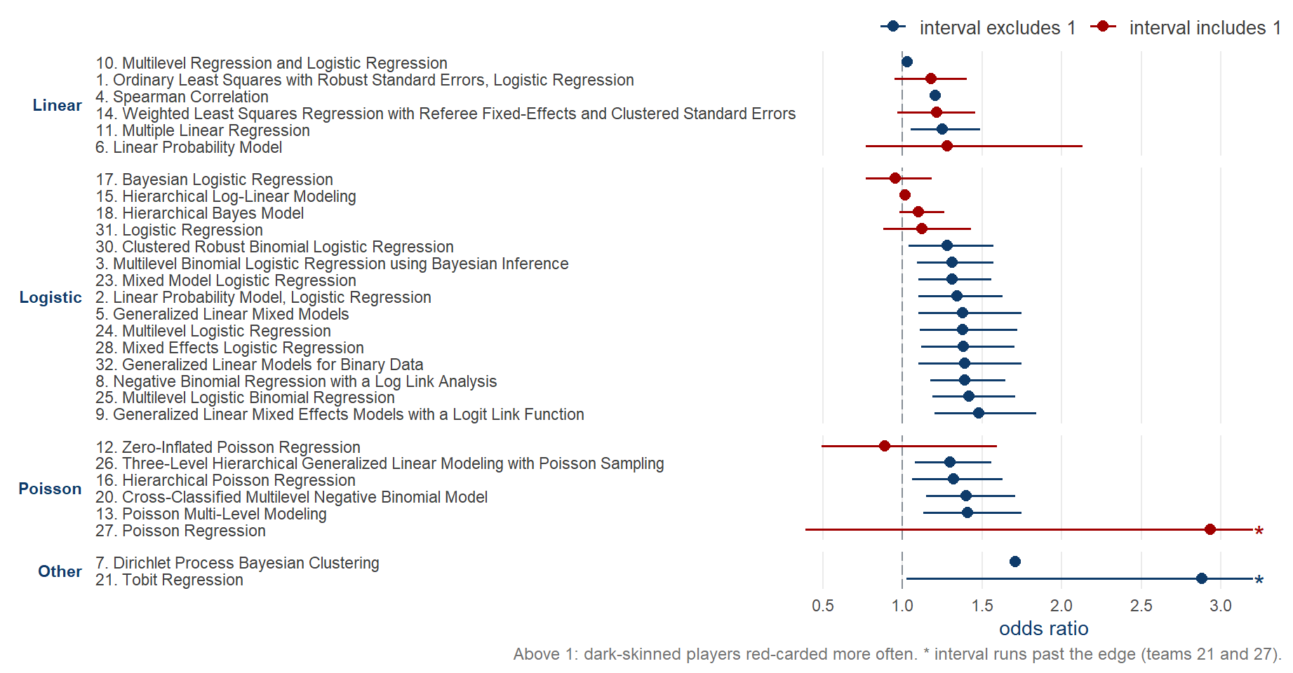
Silberzahn et al. (2018), Figure 3, rebuilt from the published values at osf.io/gvm2z.

And here is what came back. Read it as a list of twenty-nine analyses of one dataset. The odds ratios run from nought point eight nine to two point nine three – the lowest implies that dark-skinned players were red-carded slightly less often – and the median is one point three one. Twenty of the twenty-nine intervals exclude one; nine do not. So about two thirds found an effect and a third did not, on identical data. [pause] Now look at the left column. The teams are grouped by the response distribution they assumed – linear, logistic, Poisson, and two that fit none of the three. Each team made that decision for itself, and each choice was defensible. It is the same kind of decision that you will make yourselves when we reach the specification menu, where the outcome family is one of the choices.

Replication crises

Another replication crisis – terminological confusion?

The term reproducibility has been used as a synonym for a number of different characteristics – reproducibility, robustness, replicability, repeatability, credibility, and trustworthiness (Nosek et al. 2025, 2).

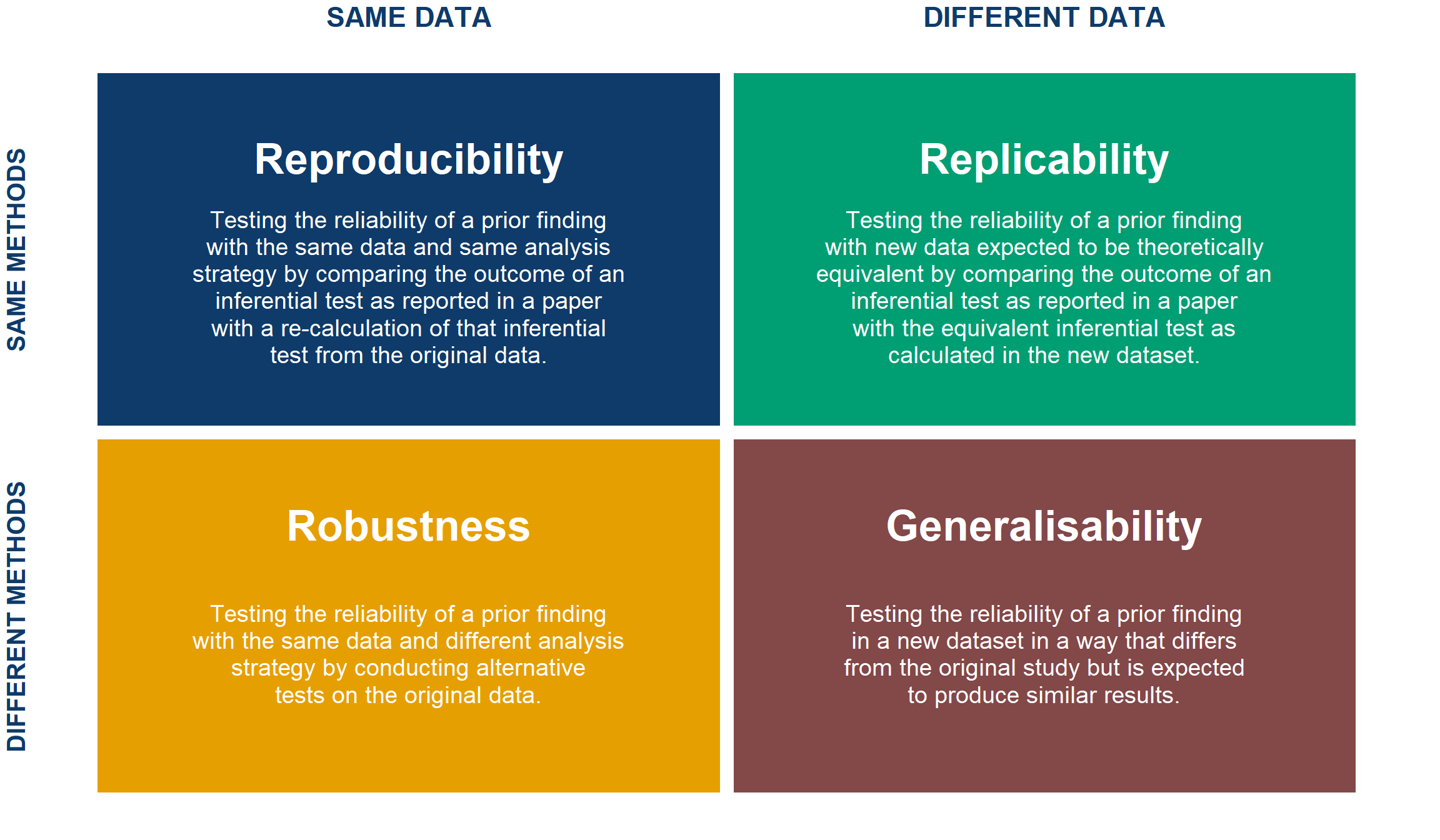
Successfully rerun the same code on the same data? Re-analyse the same data a different way? Collect fresh data and analyse it in the same way? Using the same data and same analysis but asking a different question? Asking the same question but answering it with fresh data and a different analysis?

So twenty-nine competent teams worked on one dataset and did not agree. What I have not said yet is what kind of failure that is, and part of the difficulty is the word itself. For years replication covered everything: rerunning someone’s code, re-analysing their data a different way, collecting new data altogether. Those are three different operations, answering three different questions, but because we called them all replication, the crisis debates had people talking past each other for a decade. So before any more numbers, we need the vocabulary.

The data \(\times\) analysis matrix

Alipourfard et al. (2021); Nosek et al. (2025)

Here is that vocabulary as a single grid, and if you take one thing home, make it this. The question stays the same throughout, and what varies is the data and the analysis. Same data and the same analysis is reproducibility: if I rerun your recipe, do I get your number? Same data but a different, justifiable analysis is robustness, which asks whether your finding survives my defensible choices. New data for the same question is replicability. The fourth cell, new data and new analysis, is really generalisation, and we leave it aside. Sit with the grid for a moment, because everything that follows refers back to it.

Repeatability and credibility

Repeatability is used when referring to reproducibility, robustness, and replicability as a constellation of concepts intended to assess whether answers to scientific questions are unchanged when different steps of the research process are repeated.

Credibility and trustworthiness refer to the confidence one can have in research findings. Because scientific knowledge claims are tentative, they are not synonymous with truth.

For example, credibility is advanced by addressing potential competing interests in the conducting and reporting of research, by taking existing knowledge into account, by using methods that have been validated, by controlling for biases in the research context, by pursuing precise and reliable evidence, and by calibrating the strength of the claims to the uncertainty of the evidence.

Nosek et al. (2025, 2)

The glossary on this slide is worth reading slowly, because it separates two things we routinely run together. Repeatability is the umbrella: reproducibility, robustness and replicability as a family, all asking whether the answer survives repeating some step of the process. Credibility and trustworthiness are about how much confidence a finding deserves – and note the sentence in the middle. Because scientific claims are tentative, credibility is not the same as truth. A credible finding can be wrong. What credibility is built from is the list at the bottom: declared interests, validated methods, precise evidence, and claims calibrated to the uncertainty behind them. That last one is the one we will keep coming back to.

Quick check – the matrix in peer review

You submit your paper and replication package. It goes out to reviewers.

• Reviewer 1 wants to ensure that your results are reproducible, so she sources your R script to run the entire analysis. You’re in luck – she hasn’t yet updated her dplyr, so the code runs.
• Reviewer 2 is very eager. He’s unconvinced by your modelling choices, so he fits your data to another function to check if your findings are truly robust. You’re in luck again – he recovers your point estimate to a reasonable precision, although the confidence intervals have widened.
• Reviewer 3 takes a special interest because he’s just working on a similar paper on data they published recently. Do your results replicate when your methods are applied to that state-of-the-art dataset?

Here is the matrix at work on one paper. You submit a paper with its replication package, and three reviewers each check something different. For each one, call out or type in the chat which cell of the matrix that reviewer is in, before the answer appears. Reviewer 1 reruns your own script on your own data. [pause] [advance] Reproduction. Reviewer 2 fits your data with a different function. [pause] [advance] Robustness. Reviewer 3 applies your methods to a dataset that somebody else published. [pause] [advance] Replication.

Quick check – the matrix in peer review

You submit your paper and replication package. It goes out to reviewers.

Reviewer 2 just doesn’t want to let go…

• He tried a few alternative analyses of your data, including a fancy new regression method that he just released as an R package. His method gives results that are generally aligned to yours, but for the method to work, it would require a larger dataset; would your results really generalise to this new dataset published by Reviewer 3 that he just read about, if applying his new fancy method to it?

Reviewer 2 has not finished. His new method agrees with your results, but it needs more data than you had, so he wants to run it on the dataset that Reviewer 3 published. Which cell is that? [pause] [advance] New data and a new analysis at once put him in the fourth cell, generalisation. Each of these checks asks a different question of the same paper, and passing one of them does not settle the others.

Open research: the practices

Practice	What it makes possible
Open data	Someone else can re-analyse your evidence
Open code	Someone else can rerun your exact analysis
Open materials	Someone else can run your study again
Open access	Someone else can read the claim in the first place
Preregistration	A dated record of the analysis plan, filed in a registry before the results exist
Registered reports	Peer review of the plan, with publication decided before results

Each one removes a specific obstacle, and none of them guards against every problem. The programme, set out at length: (Munafò et al. 2017)

Each of those reviewers needed something from you before they could start – your code, your data, your materials. Open research is a list of practices that supply those things and more, each of which removes a specific, identifiable obstacle. Open data means someone else can re-analyse your evidence rather than taking your word for it. Open code means they can rerun your exact analysis. Open materials means they can run the study again in a new sample. Open access means they can read the thing at all, which sounds trivial until you try to get a paper from outside a wealthy university. Preregistration produces a dated record of the analysis plan, filed in a registry before the results exist. And registered reports go further: the plan is peer-reviewed and the publication decision is made before anyone sees a result, which removes the incentive to find something. Each removes one obstacle, and none of them guards against every problem. Whether published findings hold up when somebody does check them has now been measured on a large scale.

The SCORE programme

• DARPA-funded programme to gauge the credibility of social-science claims
• A stratified sample of papers from 62 journals, published 2009–2018
• The central claim of each paper traced from the abstract to the statistic that supports it
• Thousands of researchers, and three repetition studies built on the same sampling frame

The three papers we look at next all come from one programme, SCORE, short for Systematizing Confidence in Open Research and Evidence. It was funded, oddly enough, by DARPA, the research agency of the US Department of Defense, which wanted to know whether you could predict which findings hold up. It starts from a stratified sample of papers from sixty-two journals, published between 2009 and 2018, and traces the central claim of each paper from the abstract down to the statistic that supports it. The three studies then took that same sampling frame and each asked one of our three questions. So the numbers you are about to hear all describe the same body of literature, asked three different things.

The three SCORE studies

SAME data

DIFFERENT data

SAME methods

DIFFERENT methods

Sánchez-Tójar et al. (2026)

This is the four-cell map you have just learned, but each box now shows the disciplinary breakdown from its study. Three of the four corners have a SCORE paper behind them: reproduction top-left, replication top-right, reanalysis bottom-left. The fourth, generalisation, we leave aside. Economics and political science lead on reproduction while sociology lags, replication hovers around half almost everywhere, and reanalysis holds the original conclusion three times in four. We take the three studies in turn, starting with reproduction.

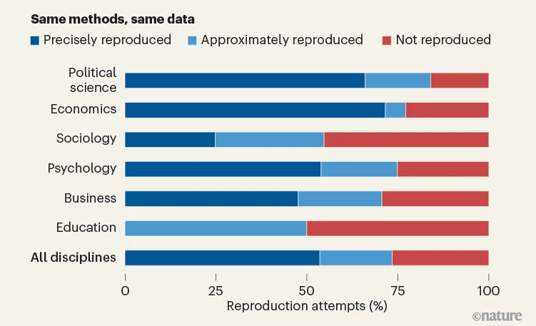
Reproducibility – Miske et al.

• 600 papers sampled (62 journals, 2009–2018)
• Ask the authors for data and code, then try to rerun the reported result
• How often is that even possible?

Miske et al. (2026).

Reproducibility is the gentlest test of the three. The design in one breath: take six hundred papers, ask the authors for their data and code, and try to recompute the central reported result from the same data with the same analysis. Before we ask how often that works, the first finding is about how rarely you can even start.

Reproducibility results – Miske et al. 

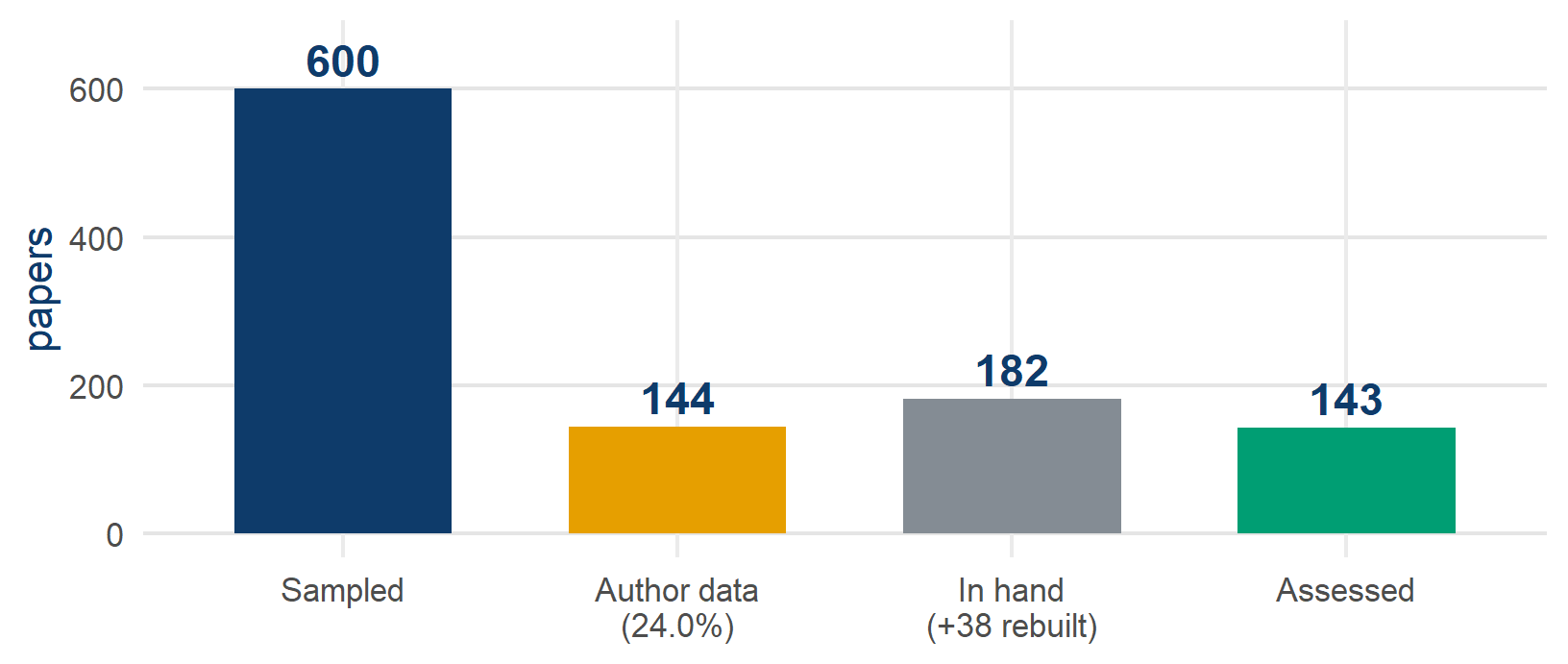
• Of the 143 assessed: 53.6% reproduced precisely, 73.5% at least approximately
• Counting the unassessable, only about 18% reproduce

Miske et al. (2026). Published counts: the 143 assessed papers come from 182 datasets, 38 of them rebuilt from source data.

Read it left to right. Six hundred papers sampled. Data were available for twenty-four per cent of them – for nearly three quarters there was neither data nor code. The team rebuilt thirty-eight more datasets from source data, which made a hundred and eighty-two, and assessed 143 of them. Of those, just over half reproduce precisely, and about three quarters at least approximately. That sounds respectable until you count the papers that nobody could check as failures, and then the overall rate falls to roughly eighteen per cent. Most of the loss happens at the first step, getting hold of the data.

Data availability – Miske et al. 

• Journals with a sharing policy: 66.2–100% data availability vs 16.0% without
• By discipline: 54.1% data availability in political science vs 2.9% in education
• With data and code: 90.9% approximately reproducible vs 38.1% from rebuilt source data

The most substantial barrier … was the unavailability of author data.

Reproducibility success does not mean that the finding is correct.

Miske et al. (2026).

And access follows policy. Where journals have a data-sharing policy, availability runs from about two thirds to one hundred per cent, depending on the policy; without one, it is sixteen. Political science and economics built the habit early and are far ahead of the rest. The first quote is the conclusion of the paper itself – the biggest barrier was simply that the data were not there. The second quote is the one to remember: reproducibility success does not mean that the finding is correct. Reproducing a number tells you that the computation was faithful, and nothing about whether the claim about the world is true.

Robustness – Aczel et al. (Multi100)

• 100 studies, each re-analysed by ≥5 independent analysts
• The same data for every analyst, each free to choose any justifiable analysis
• A peer panel judges whether each pipeline is appropriate
• I was one of its analysts

Aczel et al. (2026).

The middle paper – the one I was in. One hundred studies, and for each one at least five analysts working independently: no teams, original authors barred, everyone handed the same data and the same claim. You were free to analyse it any way you could justify, and a peer panel later judged whether your pipeline was appropriate. The hundred studies had already passed a reproducibility check, so robustness was being measured on the reproducible subset, the best-case material.

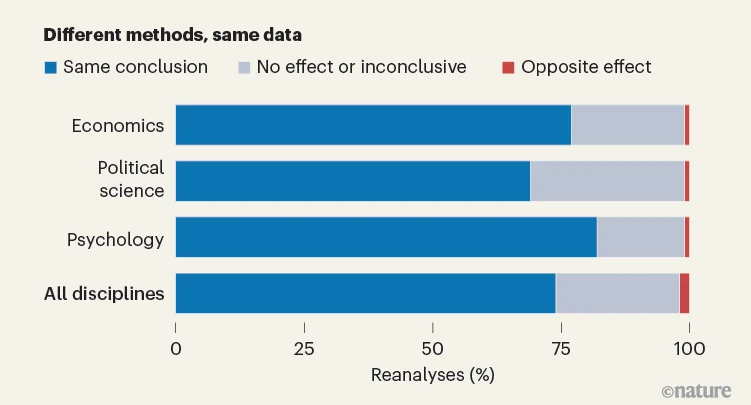
Robustness results – Aczel et al. 

• 34% of reanalysis effect sizes within ±0.05 d of the original (57% within ±0.20)
• 74% reached the same conclusion, 24% a null or inconclusive one, 2% the opposite
• Effect sizes shrank: original mean d 0.73 → reanalysis 0.49
• Analyst-to-analyst variability typically exceeds sampling error

Aczel et al. (2026).

Free, justifiable choices on the same data move the answer a long way. Only about a third of the reanalyses fell within five hundredths of a Cohen’s d of the original, and in just five studies out of ninety-five did all the analysts come that close. Conclusions held up better than magnitudes, with three quarters of reanalyses agreeing with the original conclusion. But the effect sizes shrank, from a mean d of point seven three down to point four nine. The finding I keep coming back to is that the spread across analysts is typically larger than the statistical uncertainty inside any single analysis. The analyst, in other words, is a bigger source of noise than the sample. One more detail: observational studies, which is the kind of study we work with in this course, came out less robust than experiments.

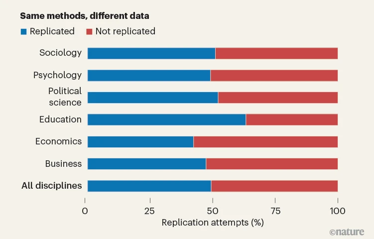
Replicability – Tyner et al.

• 274 claims from 164 papers, tested on independent data (newly collected for 128, existing for 146)
• A median statistical power of 99.6%, a preregistered protocol, and the original authors consulted
• The strictest test: does the effect reappear in data that the original study did not use?

Tyner et al. (2026).

The third paper is the strictest test, because each claim is checked against data that the original study did not use – newly collected for 128 claims, existing data for the other 146. Two hundred and seventy-four claims, each replicated to a preregistered, peer-reviewed protocol, often with the original authors consulted, and with a median statistical power of ninety-nine point six per cent. At that power an effect as large as the original one would be very hard to miss, so a claim that fails here cannot be put down to a study too small to detect it.

Replicability results – Tyner et al. 

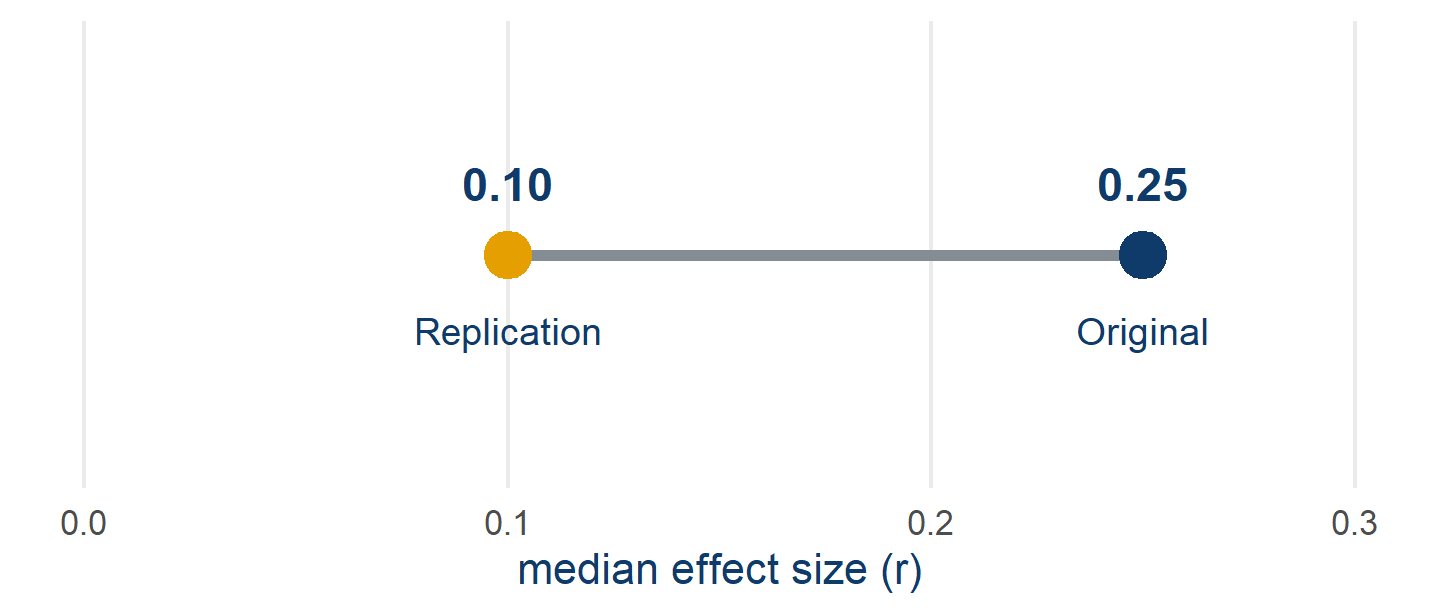
• 55.1% of claims replicated by the significance criterion, and effect sizes roughly halved
• Thirteen success criteria give anywhere from 29% to 75%

Tyner et al. (2026).

And this is what comes back. The median effect size halves: point two five in the originals, point one zero in the replications. By the significance criterion, fifty-five per cent of claims replicate. But notice that did it replicate? is not even one question – the team scored the same studies against thirteen reasonable success criteria and got answers ranging from twenty-nine to seventy-five per cent. As the paper puts it: Strictly speaking, there is no such thing as exact replication. And: The problem to solve is not unreplicability per se, it is overconfidence.

The three Rs across SCORE

Reproducible ≠ robust ≠ replicable.

Across SCORE the three are essentially uncorrelated – knowing one barely predicts the others.

So there is no single number for trust. You have to ask which repetition you mean.

You would hope these three properties go together – that a reproducible finding is more likely to be robust, and a robust one more likely to replicate. Across SCORE, and to my surprise, they do not. Measured on the same body of papers, the three indicators are essentially uncorrelated – knowing one tells you almost nothing about the others. So there is no single trust score for a finding. Is it reliable? is an incomplete question until you say which kind of repetition you mean. The claim that I was handed in the robustness study is the one this course is built on.

What a Multi100 analyst received

• A published paper, in full and not blinded, so I could see the original estimates
• Its central claim, in one sentence, lifted from the abstract
• A pointer to the data – in our case, sixteen Eurobarometer waves you fetch yourself from GESIS
• No instructions on method – any analysis you can defend

And two things I was not told: who the other analysts were, and what they were finding.

Aczel et al. (2026). Registered protocol: osf.io/7snkz

Multi100 handed a hundred published studies to at least five independent analysts each, and I was one of them. Let me show you what that was like from the inside, because it shapes how you read the results. What arrived was a published paper – the whole thing, not blinded, so I could see the original estimates, and if anything that pulls you towards the original answer. With it came the central claim of the paper in a single sentence, lifted from the abstract, and a pointer to where the data were held. In our case that meant sixteen Eurobarometer waves that I had to go and fetch from GESIS myself, under licence. What did not arrive was any instruction on method. Analyse it however you can defend. And two things stayed hidden throughout: who the other analysts were, and what any of them were finding. The isolation was part of the design, because it is what makes the spread at the end mean something.

The paper in brief

• Author: I will say OA, the original author, from here on
• Does the EU economic crisis undermine support for the EU? – 16 Eurobarometer waves, 2004–2013, about 390,000 respondents in 27 countries

The results show, first, that poor economic performances increase negative and decrease positive dimensions of EU framing.

• Macro predictors: national unemployment and GDP growth. Outcome: what people say the EU means to them, sorted into four framing scales

Teney (2016). The full methodological reading comes later in the course.

And here is the paper, briefly. We come back to it later and spend a long time inside it, so this is just enough to follow what happened. It is from 2016, in the European Sociological Review, and I will call its author OA, the original author, from here on. The question is whether the economic crisis undermined how people relate to the EU: sixteen Eurobarometer waves from 2004 to 2013, the crisis decade, about three hundred and ninety thousand respondents across twenty-seven member states. The claim we were handed is the sentence in the box. On the right-hand side sit two macro indicators, national unemployment and GDP growth; on the left, what people say the EU means to them personally, sorted into four framing scales. That is all you need for now, and when we return to the paper we take the whole thing apart.

The two Multi100 tasks

Task 1 – free reanalysis. Reanalyse the claim however you see fit. Record one categorical conclusion: does the evidence support it?

Task 2 – constrained reanalysis. Months later, three instructions arrive that fix the question:

• use the cosmopolitan framing dimension as the outcome
• use the unemployment rate as the predictor
• disregard the contextual variables

Task 1 measures whether we agree. Task 2 makes our numbers comparable – you cannot average five answers to five different questions.

The study ran in two stages, and the distinction matters for everything that follows. Task one was complete freedom: reanalyse the claim however you see fit, and record one categorical conclusion on whether the evidence supports it or not. Then months later, task two arrived with three instructions that pinned the question down. Use the cosmopolitan framing dimension as your outcome, use the unemployment rate as your predictor, and disregard the contextual variables. The order matters because the two tasks measure different things. Task one asks whether independent analysts reach the same verdict. Task two asks whether they produce the same number, and you can only ask that second question once everyone is answering the same question, which is what those three instructions secured.

Results on a common scale

• Every analyst reports their test statistic and its degrees of freedom, in whatever form their model produces – t, z, F, \(\chi^2\)
• Each is converted to a partial correlation r and a standardised Cohen’s d, so a pooled model fitted in Stata and a multilevel model fitted in R can be read on the same axis
• A peer panel judges whether each pipeline is an appropriate analysis of the claim
• Only then can you ask: how far apart are five defensible answers?

Standardising makes the comparison possible, but it assumes that the five are estimating the same quantity. Hold that thought until we come to estimands.

Even with the question pinned down, the answers arrive in different forms. Everyone reports the test statistic that their model happens to produce, with its degrees of freedom – a t, a z, an F, a chi-squared. Those get converted onto a common scale: a partial correlation and a standardised mean difference, so that somebody’s pooled Stata model and somebody else’s R multilevel model can be placed on the same axis and read against each other. Alongside that, a peer panel judged whether each pipeline was an appropriate analysis of the claim at all – so the spread you are about to see is a spread among analyses that passed review. Putting five numbers on one axis, though, takes for granted that they estimate the same quantity. Hold on to that, because when we come to estimands, much of the argument is about what happens when they do not.

The five analysts – Task 2 results

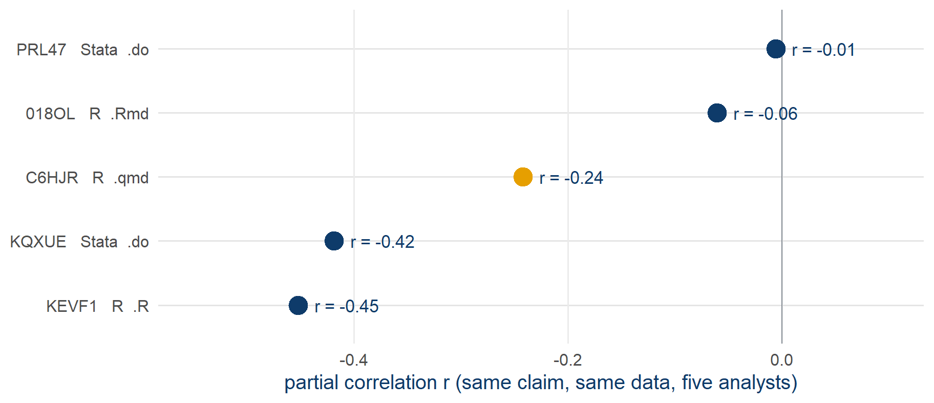
• All five estimates negative, with partial r from −0.45 to −0.006, and one of them not significant

Task 2 results as recorded in the public Multi100 dataset (osf.io/q5h2c).

And here are the five of us, on this one claim. All five found a negative effect, so on direction we were unanimous. On size, look at the spread: from essentially zero, and that one is not significant, out to a partial correlation of minus point four five. That is two orders of magnitude, on the same data and for the same claim, with all three Task 2 instructions obeyed. The orange dot is me, at minus point two four. Before we go anywhere near why, which takes much of the rest of the course, I want you to look at the labels down the left-hand side, because there is a column there that I have not mentioned yet.

Software and document formats

• Two of us worked in Stata, three in R
• Within R, three different document formats: a plain .R script, an .Rmd, a .qmd

The software did not cause the spread. There is no Stata answer and no R answer to this claim.

But because each of us submitted a document that somebody else could open and run, it became possible, afterwards, to find out what did cause it.

That is what the toolchain is for.

Two of the five worked in Stata, three in R – and within R, three different document formats: a plain script, an R Markdown file, a Quarto file. Now, the tempting reading of that column is the wrong one, so let me rule it out straight away. The software did not cause the spread. There is no Stata answer and no R answer to this claim; every one of these models can be fitted in either. But the column does matter, and it is why the tooling is worth caring about. Because every one of us submitted a document that somebody else could open and run, it became possible afterwards to go and find out what actually did cause the spread. I have read the code of all four of the others, line by line, and later you will work through the same choices that they faced. That is only possible because of what is in that column. So – the tools.

Open-source software

• You can read it. The source of lm(), of feols(), of every package that this course loads, is public, so no estimator has to be taken on trust
• No licence stands between a reader and your analysis. Anyone, anywhere, can run your code without buying anything
• It outlives your institution. A licence expires when you change job; a package on CRAN does not
• You can fix it, and so can others. Bugs get found because thousands of people run the same code on different data

With a proprietary toolchain, the price of reproducing your work falls on your reader, who has to buy the licence.

Stata is proprietary and R is open source, and that difference matters for reproduction. There are four reasons, and only one of them is money. First, you can read it. You can go and look at the source of any function we run in this course, so you never have to take an estimator on trust. Second, and this is the one that bears on our subject, no licence stands between a reader and your analysis. If your replication package needs a licence they do not have, your work is not reproducible for them, however carefully you wrote it. Third, it outlives your institution – a site licence ends when you change job, and a package on CRAN does not. Fourth, bugs get found, because thousands of people run the same code against different data. On money, the question is who pays. Reproducibility has a price, and a proprietary toolchain hands that price to your reader.

The toolchain

Analyse

Rstatistics-first language

Pythongeneral purpose, good for machine learning

Juliafast numerics

Stata / SPSSproprietary, still standard in places

Write

Positronthe course default

RStudiothe familiar one

VS Codeeverything, via extensions

Jupyternotebooks, Python-first

Publish and share

Quartotext + code → anything

Gitevery version, dated

GitHubwhere the repository is hosted

OSF / Zenodoarchive with a DOI

Ringed in orange: the tools that this course uses. The others are there so that you know what you are choosing between.

The whole set of tools fits on one slide once you sort it by job rather than by brand family. First, something to analyse with – R, which is what we use, but Python and Julia are entirely reasonable choices for this work, and Stata and SPSS are still the default in a lot of departments. Second, somewhere to write it: Positron is what I will be driving on the shared screen, RStudio is the one most of you will already know, VS Code does everything if you are willing to configure it, Jupyter is the notebook world. Third, publishing and sharing, which is the part that people skip. Quarto turns text and code into a document; git records every version with a date; GitHub hosts the repository so others can reach it; and OSF or Zenodo give the whole thing a permanent address with a DOI. Ringed in orange is what this course uses, and the rest is there so you know the alternatives.

Programming languages

RBuilt by statisticians for data analysis. Hard to beat for models, tables and figures, thanks to its packages.

PythonA general language that also does data. Better for pipelines, scraping, text and machine learning.

JuliaFast, young, small ecosystem. Worth it when your model takes hours.

StataExcellent panel and survey estimators, superb docs, one syntax. Costs money and hides its source.

You do not have to choose once and forever. Quarto runs R, Python and Julia chunks in the same document, and the course browser lab is R compiled to run inside a web page.

A slower look at the languages, because people agonise about this and mostly should not. R was built by statisticians for data analysis, and that is still where it wins, in models, tables and figures. Most of that comes from the package ecosystem: whatever obscure estimator your literature uses, someone has written the package. Python is a general-purpose language that also does data, so it is the better choice for pipelines, scraping, text and machine learning. Julia is fast and young with a small ecosystem, and earns its place when a model takes hours rather than seconds. Stata deserves respect – excellent panel and survey estimators, the best documentation in the business, one consistent syntax – and it costs money and hides its source. And none of this is a life choice, because Quarto will run R, Python and Julia chunks in the same document.

Editors and IDEs

PositronThe newer IDE from Posit. R and Python as equals, VS Code underneath.

RStudioStill excellent, still supported. If it is what you know, use it.

VS CodeDoes anything, once configured. Big extension ecosystem.

JupyterNotebook-first. Beware: cells can run out of order.

NeovimFor the keyboard-only. Steep to learn, and very fast once learned.

Of the choices in the toolchain, the editor matters least. It changes how you work and nothing about what a reader receives.

A trap: a notebook lets you run cells out of order, so it can show output that no clean run would produce. Restart and run everything before you believe it.

Positron and RStudio are both from Posit; both are free, and RStudio is open source.

The editor is the least consequential choice in the toolchain, so I will be quick. Positron is the newer environment from Posit, built on VS Code, treating R and Python as equals – it is what I will be driving on the shared screen. RStudio is still excellent and still supported, and if it is what you know, there is no reason to move. VS Code will do anything once you have configured it. Jupyter is notebook-first and Python-first. Neovim is for people who never want to touch a mouse. What matters is the trap in the second box, and it applies to every notebook-style tool including the interactive mode in Quarto: you can run cells out of order, which means the output on your screen may be output that no clean run would ever produce. Restart the session and run everything, top to bottom, before you believe a number.

Plain-text file formats

.RCode only, with prose in comments.

.mdProse only. Headings, lists, links – no code.

.RmdProse + R, rendered together. R only.

.qmdProse + R, Python or Julia. The course format.

Every one of these is a plain text file. You can open it in anything, compare two versions of it line by line, email it, and read it in twenty years. A .docx with pasted output is not plain text, and nothing in it records which numbers came from which code.

Four file types, in increasing order of what they hold. A dot-R file is code with comments. A markdown file is prose with no code. An R Markdown file is prose and R together, rendered into one document. And a Quarto file is the same idea, except the code can be R or Python or Julia. What they have in common is that every one is a plain text file. You can open it in any editor, see exactly what changed between two versions, email it, and still read it in twenty years. Compare that with a Word document holding numbers you pasted in from somewhere. It looks the same on the page, but nothing in it records which number came from which line of code. That is how the old value of a number you have since recomputed can still be sitting in the paper.

What happens when you render

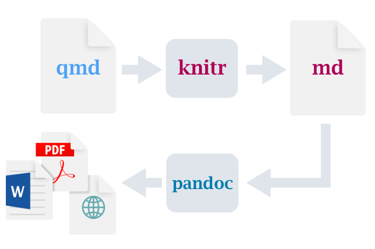
You write one source file. Rendering runs your code, inserts the results, and produces whatever output you asked for from that one source.

And this is what happens when you press render. You write one source file, with prose and code together. Knitr – or Jupyter, if you are working in Python – runs every chunk of code in a fresh session and replaces it with its actual output, giving a plain markdown file. Pandoc then turns that into whatever you asked for: a Word document for your co-author, a PDF for the journal, a web page for your project site, slides like these. So there is one place where a number is computed, and every output shows the same number, because they were all produced from the same source in the same run. When a reviewer asks you to drop three countries, you change one line and re-render, and the table, the figure and the sentence in the text all change together. That alone makes rendering worth learning, quite apart from anything to do with credibility.

The package layer

tidyverseReading, reshaping, plotting. One grammar across all of it.

easystatsModel output as tidy data: parameters, performance, effect sizes.

modelsummaryRegression tables you can publish, from the fitted objects.

marginaleffectsPredictions, contrasts and marginal effects from almost any model.

The tasks also use fixest (fast fixed effects – the estimator behind our baseline), dagitty and ggdag (causal graphs). The full setup is on the setup page, and the check script in your workspace reports whether all three are installed.

A word about packages, because this is where the advantage of R actually lies. The tidyverse gives you one consistent grammar for reading data, reshaping it and plotting it, so once you have learned the verbs they work everywhere. Easystats turns model output back into tidy data – coefficients, fit statistics, effect sizes – instead of the printed blob that summary gives you. Modelsummary builds publication-ready regression tables straight from fitted model objects, so your table cannot disagree with your model. And marginaleffects computes predictions, contrasts and marginal effects from almost any model you can fit, which is how you get from a coefficient to a statement in the units that your reader thinks in. The tasks also use fixest for fast fixed effects – that is the estimator behind our baseline – and dagitty and ggdag for the causal graphs. The check script in your workspace reports whether those three are installed.

Version control

Git is a program on your machine. It records a complete, dated snapshot every time you say so, and it never forgets one.

GitHub is a website that hosts those snapshots so other people can reach them – and it is not the only one (GitLab, Codeberg, one hosted by your university).

What it gives you that a folder of final_v3_REALLY_final.R cannot:

• Every past state, recoverable exactly
• A written reason attached to each change
• A public, timestamped trail of when you knew what
• A way for two people to edit the same file without one overwriting the other

The tasks use none of it. There is a companion module on the site, and your workspace folder is the ideal thing to practise on.

Version control is the one tool that I have kept out of the tasks, so let me at least name it properly. Git is a program that runs on your machine: every time you tell it to, it records a complete dated snapshot of your project, and it never forgets one. GitHub is a website that hosts those snapshots so other people can reach them. It is not the only one: there is GitLab, there is Codeberg, and your university may run its own. What does that give you that a folder full of final-version-three-really-final does not? Every past state recoverable exactly, a written reason attached to every change, a public timestamped trail of when you knew what – which, notice, is a preregistration mechanism in itself – and a way for two people to work on one file without one silently overwriting the other. There is a companion module on the site.

Where data and code are archived

OSFProjects, files, and registrations. Free, and it hosts the public record of our case.

ZenodoCERN-run archive. Gives a DOI; takes a GitHub release directly.

DataverseInstitutional data archives with proper metadata and curation.

XYZDomain archivesGESIS, UK Data Service, ICPSR – licensed access to survey microdata.

A repository is not an archive. A GitHub repository can have its history rewritten, be renamed, or be deleted tomorrow. An archived deposit gets a DOI, a fixed version, and a commitment to keep serving it. Serious work usually needs both.

And the last group: where things go so they are still there in ten years. OSF is free, holds projects and files and registrations, and the whole public record of our case is kept there – you will be reading it later. Zenodo is run by CERN, gives you a DOI, and will take a GitHub release directly, which makes archiving a one-click habit. Dataverse is the institutional data-archive world with proper metadata and curation. And then the domain archives – GESIS, the UK Data Service, ICPSR – which is where licensed survey microdata is held, including the Eurobarometer data behind our paper. A repository is not an archive, although people often treat it as one. A GitHub repository can have its history rewritten, be renamed or be deleted tomorrow, and the link in your paper dies. An archived deposit has a DOI, a fixed version and an institution committed to serving it. Serious work usually needs both.

Licences, briefly

What	Common choice	Why
Code	MIT · GPL	MIT: use it however you like. GPL: and share your changes back
Data	CC0 · CC BY	CC0 puts it in the public domain; CC BY asks for attribution
Text, figures, slides	CC BY · CC BY-NC	Attribution, optionally no commercial reuse
Someone else’s data	their terms	Eurobarometer is GESIS-licensed – I may not redistribute it, and neither may you

Publishing with no licence is not a neutral default. It means all rights reserved – legally, nobody may reuse the work at all.

Licensing gets skipped and then bites. Four rows. For code, MIT says use it however you like, GPL says use it and share your changes back. For data, CC-zero puts it in the public domain and CC-BY asks for attribution. For text and figures and slides, CC-BY or CC-BY with a non-commercial clause. And the fourth row is the one that constrains this course: when the data are not yours, their terms govern. The Eurobarometer microdata behind our paper is GESIS-licensed – I am not allowed to redistribute it, which is why you will be working on an aggregate I built and am allowed to share, and it is also the reason why the first SCORE attempt to reproduce this paper failed, which we come back to when we reach the paper itself. And the line at the bottom: leaving a repository without a licence does not make it free to use. Legally it means all rights reserved, so nobody may reuse it at all.

The workspace and the browser lab

Your IDE and the workspace

• The workspace folder you downloaded, opened in your IDE (Positron, RStudio, VS Code, etc.)
• Quarto renders your report; fixest fits your models
• No git, no cloning, no configuration – it is just files
• This is what I drive on the shared screen

The browser lab

• One web page. R is compiled to run inside the browser
• Nothing installed, nothing to break, data already in place
• The same tasks, data and helpers, on the shared screen and in your own tab
• Your spare if your installation misbehaves at any point

github.com/CodeMoreh/replication-lab – download zip → unzip → open in your IDE

This is what you will actually be working in. The workspace is the folder you downloaded, open in your IDE, which is Positron on my screen and may be RStudio or VS Code on yours. Quarto renders your report, fixest fits your models, and there is no git and no cloning because it is just a folder of files. That is what I will be driving on the shared screen, so you can follow keystroke for keystroke. The browser lab is one web page with R compiled to run inside the browser itself. Nothing installed, nothing to break, and the data are already there. Every task exists in both, with the same data and the same helper functions, so you can switch at any point if your machine misbehaves, and several people usually do. The address for the workspace zip is at the bottom, and it is on the setup page in the chat.

What the tools cannot do

A perfectly reproducible pipeline can be a perfectly reproducible answer to a question you never stated.

None of this software will tell you what your estimand is, whether your controls belong in the model, or whether the association you found means what you think it means.

Tooling is the cheap half of the problem, because it can be learned. The expensive half is the question that the analysis is meant to answer.

All of this software is worth having, but a perfectly reproducible pipeline can be a perfectly reproducible answer to a question you never stated. None of this software will tell you what your estimand is, whether the variables you put in the model belong there, or whether the association you found means what you think it means. Tooling is the cheap half of the problem, in the sense that it can be solved by learning things. The expensive half starts from a question that every quantitative study has to answer, namely what exactly you are trying to estimate, and a good deal of what follows is about that question. First, though, you need a setup that works.

Hands-on 1 – The setup check

Task 1 – the setup check. Get to the point where a line of R runs and the data are in front of you.

• Workspace: your IDE opens the workspace folder, the packages install, working_script.R runs its first block, and the report skeleton renders
• Browser lab: the page has finished loading, the first chunk runs, and euframes has 270 rows

Take the time you need, into the next break if necessary. Type a green circle in chat when you are through; type STUCK and I will come to you.

If your installation will not cooperate, do not fight it – open the browser lab and carry on. Nothing in the tasks depends on which one you use.

Right – your turn, and this first one is deliberately not intellectual. The job is to get to the point where a line of R runs and the data are in front of you. For the workspace, open the workspace folder in your IDE, let the packages install, run the first block of the working script, and render the report skeleton once so you know it works. In the browser lab, wait for the page to finish loading, run the first chunk, and check that the panel has two hundred and seventy rows. Take the time you need over it, into the next break if you have to. There is no prize for finishing early, and getting this right now saves an hour of misery later. Green circle in chat when you are through, STUCK if you need me. And if the workspace will not cooperate, do not fight it. Switch to the browser lab and carry on – nothing in the tasks depends on which one you use.

R, in one slide

R tutorial · 10 slides · skip to Hands-on 2 →

x <- 42                          # <- assigns. "x gets 42"

mean(c(2, 4, 6))                 # a function: name, then arguments in ()

euframes$unemp                   # $ picks one column out of a data frame

euframes |> nrow()               # |> the pipe: send the left into the right

With four pieces of syntax you can read most R: assign with <- · call a function with name(...) · reach into an object with $ · chain with the pipe |>.

If you have never written a line of R, this slide is most of what you need to read the rest. Four things. First, the arrow assigns: x gets forty-two. You will see the equals sign used the same way and both work, but the arrow is the convention and it reads better out loud. Second, a function is a name followed by round brackets containing its arguments – mean of two, four and six. Third, the dollar sign reaches inside an object to pull out one column. And fourth, the pipe, which is the one that changes how the code reads: it takes whatever is on its left and feeds it in as the first argument of whatever is on its right. So euframes pipe nrow means take euframes, and count its rows. Once you see the pipe as the word then, long chains become readable sentences.

Getting data in

library(readr)                                # load a package

euframes <- read_csv("data/EUframes_cy.csv")  # read it, name it

euframes                                      # print it

What comes back is a data frame: a rectangle, one row per observation, one column per variable, each column of a single type. Almost everything in R takes a data frame and gives you one back.

library() makes the functions in a package available. It does not install it – that is install.packages(), and it happens once, not every time.

Getting data in. The library line makes the functions in a package available for this session – and note that it does not install anything; installing is a separate thing you do once. Then read underscore csv reads the file and the arrow gives the result a name, so from here on euframes is our panel. Typing the name on its own prints it. What you get back is a data frame, which is the central object in R: a rectangle with one row per observation, one column per variable, and each column holding a single type. Nearly every function you will meet takes a data frame and hands you a data frame back, which is why the pipe works so well – the output of one step is the right shape to be the input of the next.

Inspecting the data

glimpse(euframes)      # every column, its type, the first few values
nrow(euframes)         # 270
summary(euframes$unemp)  # min, quartiles, mean, max

euframes |>
  count(cntry)         # how many rows per country?

Every serious error I have made in twenty years of this was visible in the data before it reached a model – a duplicated year, a missing value coded as -9, a scale running 1–10 where I assumed 0–1.

With the panel loaded, the next step is to look at it before any model touches it. Glimpse shows every column with its type and first few values. nrow counts the rows. Summary on a single column gives the minimum, the quartiles, the mean and the maximum. And count, piped, tells you how many rows there are per country – which for a balanced panel should be the same number every time. Then the fragment. Every serious error I have made in twenty years of doing this was visible in the data before it ever reached a model: a year that appeared twice, a missing value coded as minus nine and quietly averaged in, a scale running one to ten when I had assumed nought to one. Ten minutes of looking pays back more than any other ten minutes in the workflow, and it is the part that people skip because it does not feel like analysis.

Working with rows and columns

euframes |>
  filter(year >= 2008) |>                       # keep some rows
  select(cntry, year, mcosmo, unemp) |>         # keep some columns
  mutate(unemp_c = unemp - mean(unemp)) |>      # make a new column
  arrange(desc(unemp))                          # sort

Read it downwards as a sentence: take the panel, then keep 2008 onwards, then keep four columns, then add a centred unemployment column, then sort by unemployment, highest first.

The sixth verb is summarise(), usually with group_by(): collapse many rows into one per group. That is how the panel you are working on was built from 390,000 respondents.

Five verbs get you a very long way, and they all share one pattern: first argument a data frame, result a data frame. Filter keeps rows. Select keeps columns. Mutate makes a new column. Arrange sorts. And the pipe strings them together so you read the whole thing downwards as a sentence: take the panel, then keep 2008 onwards, then keep these four columns, then add a centred unemployment column, then sort by unemployment with the highest first. The sixth verb, on the fragment, is summarise, usually paired with group-by: collapse many rows into one row per group. I mention it because it is the operation that produced the panel you will be working on – three hundred and ninety thousand respondents collapsed into two hundred and seventy country-year means.

Model formulas

mcosmo ~ unemp                    # "mcosmo explained by unemp"

m <- lm(mcosmo ~ unemp, data = euframes)

summary(m)

The tilde ~ reads outcome on the left, predictors on the right. Add predictors with +. The formula is an object in its own right and is not tied to the function that will eventually use it.

Almost every modelling function in R takes this same shape: something(formula, data = ...). Learn the pattern once and lm, glm, lmer, feols and betareg all become variations.

A model in R is a formula plus data, and the tilde is the heart of the formula: outcome on the left, predictors on the right, and you add more predictors with a plus. The thing that surprises people coming from other software is that the formula is an object in its own right – you can store it in a variable, print it, pass it around – and it is not tied to the function that will eventually use it. Then lm fits a linear model given that formula and a data frame, the arrow names the result, and summary prints the coefficient table. The genuinely useful pattern is on the fragment: almost every modelling function in R has this same shape, something bracket formula comma data. Learn it once and lm, glm, lmer for multilevel models, feols for fixed effects and betareg for bounded outcomes all become variations on one thing you already know.

Fixed effects with fixest

library(fixest)

m1 <- feols(mcosmo ~ unemp_c | cntry + year, data = euframes)

The bar | separates the regression from the fixed effects. Everything after it is absorbed: cntry gives every country its own intercept, year gives every year its own.

The equivalent with dummies would be mcosmo ~ unemp_c + factor(cntry) + factor(year) – same estimate, 36 extra rows of output you do not want to read.

This is the model that you reproduce in Hands-on 3, where it gives t = −3.804.

This is the line that you will run yourself when you reproduce the result of my Multi100 reanalysis, so it is worth a slow look. Feols comes from the fixest package and fits linear models with fixed effects very fast. The bar is the key piece of syntax: everything to the left of it is the regression, everything to the right is absorbed as fixed effects. Country gives every country its own intercept, so we are comparing each country with itself over time rather than comparing countries with each other. Year gives every year its own intercept, so anything that hit all of Europe in a given year is soaked up. You could write the same model with dummy variables – the estimate would be identical – but you would get thirty-six extra rows of output that nobody wants to read. And in the third hands-on this same line gives a t of minus three point eight zero four.

Reading what comes back

broom::tidy(m1)
#> term      estimate    std.error   statistic   p.value
#> unemp_c   -0.00347    0.00091     -3.80       0.00019

• estimate – a one-point rise in unemployment goes with a fall of 0.00347 on a 0–1 framing scale
• std.error – how much that estimate would wobble across repeated samples
• statistic – the t: the estimate divided by its standard error. Roughly, how many standard errors from zero
• p.value – how often you would get a t this large if the true value were zero

broom::tidy() returns the table as a data frame, so you can filter it, join it, plot it. That is how 840 model fits become one chart when we reach the multiverse.

And what comes back. The tidy function from broom turns the model into a small table. The estimate says a one-point rise in the unemployment rate goes with a fall of about three thousandths on a nought-to-one framing scale – small, but the scale is small too, which is why we will standardise later. The standard error says how much that estimate would move across repeated samples. The statistic is the t: the estimate divided by its standard error, which you can read as how many standard errors the estimate is from zero. And the p-value says how often you would get a t that large if the true value were zero. Now the fragment. Tidy hands the table back as a data frame. That means you can filter it, join it, stack hundreds of them and plot the lot – and that is how eight hundred and forty model fits become one chart when we reach the multiverse.

Plotting with ggplot2

ggplot(euframes, aes(x = year, y = mcosmo)) +   # data, and what maps to what
  geom_line(colour = "grey55") +                # draw lines
  geom_point(size = 0.7) +                      # and points
  facet_wrap(~ cntry)                           # one small panel per country

Three parts, always: the data, the mapping (aes) from variables to visual properties, and one or more geoms that draw something. Layers stack with +.

facet_wrap repeats the whole plot once per group. One line of code gives twenty-seven small country panels, and you can see which countries move.

Plotting, briefly, because you will use it in the next task. Ggplot always has three parts. The data. The mapping – that is what aes does – saying which variable becomes which visual property, here year on the horizontal and cosmopolitan framing on the vertical. And then one or more geoms that actually draw something, stacked with plus signs: lines, then points on top. The one worth stealing is on the fragment: facet-wrap repeats the entire plot once per group, so that single line gives you twenty-seven small country panels side by side. That is the plot you will make in the next task, and I want you to actually look at it rather than skip past it, because you can see with your eyes which countries move sharply around 2009 – and that is the variation that the fixed-effects model is using.

Causal graphs in R

dag <- dagify(
  framing ~ unemployment,          # unemployment -> framing
  framing ~ country + year,        # country and year -> framing
  unemployment ~ country + year,   # ... and -> unemployment
  exposure = "unemployment",
  outcome  = "framing")

adjustmentSets(dag)                # what must I control for?

Each line is one arrow, read outcome-first, following the same convention as a model formula. Because every arrow has its own line, you can comment one out with a # and the code still runs.

adjustmentSets() returns the variables that close every back-door path in the graph. Change an arrow, rerun, and watch the answer change.

The last piece of R is the one you use in the next task. A causal graph in R is a set of formulas, and they follow the same convention you already learned for models: outcome on the left, cause on the right. So the first line says unemployment points at framing. The second says country and year both point at framing. The third says they also both point at unemployment – which makes them common causes, which makes them confounders. Then you declare which node is the exposure and which is the outcome. The lovely part is that each arrow is its own line, so you can put a hash in front of one and the code still runs, and wiring your beliefs into the graph is literally a matter of commenting lines in and out. [advance] And adjustmentSets reads the finished graph and tells you which variables you must control for. Those are the variables that close every back-door path, a term that the causal-graph slides explain. Change an arrow, rerun it, watch the answer change.

Common error messages

What you see	What it usually means
could not find function "feols"	The package is not loaded – add library(fixest) above
object 'euframes' not found	You ran this chunk before the one that creates it – go back up and run in order
object 'unemp_c' not found	The column does not exist yet – you skipped the mutate() that makes it
+ on the console, nothing happens	An unclosed bracket or quote. Press Esc and look for the missing )

Read the error. R error messages are terse but almost always literally true, and most of them name the thing that R could not find.

These four errors will be about ninety per cent of what you hit in the tasks. Could not find function means the package is not loaded – add the library line above it. Object euframes not found means you ran a chunk before the one that creates the object, so go back up and run them in order, and this is the notebook trap, where cells run out of order. Object unemp underscore c not found means you skipped the mutate line that makes the column. And if the console is showing you a plus sign and nothing is happening, R thinks you have not finished the command – there is an unclosed bracket or quote somewhere. Press Escape and go looking for it. The general advice is on the fragment, and it is the habit I would most like you to keep: read the error. R error messages are terse and unfriendly, but they are almost always literally true, and most of them give you the exact name of the thing that R could not find.

DAY 2 · PART 1 – The claim and its estimand

Day 2 · Part 1 · sessions 1 and 2

Day two, and the workshop day proper. Yesterday covered the credibility argument and the toolchain, so today opens straight on the paper: in full, then the argument that analysts who look as though they disagree are answering different questions, the causal-graph crash course, and your own estimand and graph. This part runs across the first two sessions of the day, because the graph work is not to be hurried.

The original paper

• 16 Eurobarometer waves, 2004–2013; about 390,000 respondents in 27 countries

The results show, first, that poor economic performances increase negative and decrease positive dimensions of EU framing.

• What does the EU mean to you personally?
  • COSMOPOLITAN: positive non-materialist form of EU framing (Peace; Democracy; Freedom to travel, study and work anywhere in the EU; Cultural diversity; Stronger say in the world)
  • UTILITARIAN: positive materialist form of EU framing (economic prosperity and social protection)
  • COMMUNITARIAN: negative non-materialist form of EU framing (Loss of our cultural identity; More crime; Not enough control at external borders; Unemployment)
  • LIBERTARIAN: negative materialist form of EU framing (Bureaucracy; Waste of money)

Teney (2016).

Back to OA’s paper, and this time properly. Sixteen Eurobarometer waves, 2004 to 2013 – the crisis decade – with about three hundred and ninety thousand respondents across twenty-seven member states. The outcome comes from one rather good survey item: what does the EU mean to you personally? It offers thirteen response options, which OA organises into four framing scales, and those are worth reading slowly, because every task from here on depends on them. Cosmopolitan is the positive non-materialist one: peace, democracy, freedom to travel and study and work anywhere, cultural diversity, a stronger voice in the world. Utilitarian is positive and materialist, covering prosperity and social protection. Communitarian and libertarian are the negative pair. The sorting into four scales is itself a substantive theoretical claim about what the EU means to people, and one you could argue with, which several of you will do in the tasks.

The claim card, as analysts received it

… poor economic performances … decrease positive dimensions of EU framing

Teney (2016: 619)

• Published coefficient – unemployment → cosmopolitan framing, Table 3 Model 1:
• b = −0.00340 · t = −4.03 · p < .001

This is the claim that every Multi100 analyst was handed, the sentence from the previous slide cut down to its positive half: poor economic performances … decrease positive dimensions of EU framing. And this is the published number behind it, from Table 3, Model 1 – the unemployment coefficient on cosmopolitan framing: minus point zero zero three four, t of minus four.

The model OA fitted

• The unit is a person, not a country-year: roughly 390,000 respondents
• Thirteen response options collapse into four framing scales – cosmopolitan, utilitarian, communitarian, libertarian
• A three-level model: respondents inside country-waves inside countries
• Individual covariates: sex · age · education band · occupational status · urbanisation · left–right placement
• Macro predictors: unemployment rate and GDP growth, entering at the country-wave level
• Plus cross-level interactions – does the macro effect differ by education?

Published coefficient, Table 3 Model 1 – unemployment on cosmopolitan framing: b = −0.00340 · t = −4.03 · p < .001

Teney (2016).

That coefficient comes out of a much larger model. OA’s unit of analysis is the person, around three hundred and ninety thousand of them, rather than the country-year. The outcomes are the four framing scales you have just met. The model has three levels: respondents inside country-waves inside countries. At the individual level sit the usual controls – sex, age, education band, occupational status, urbanisation and left–right placement. The two macro predictors, unemployment and GDP growth, enter at the country-wave level, and cross-level interactions ask whether the macro effect differs by education. [advance] The number on the claim card is one coefficient from that model, unemployment on cosmopolitan framing in Table 3, Model 1, which is minus point zero zero three four, with a t of minus four.

Model 1 and Model 2

• Model 1: unemployment → cosmopolitan framing · b = −0.00340 · t = −4.03 · p < .001
• Model 2: the same coefficient, with further controls added – drops by more than half and loses significance

Within one paper, support for the claim depends on which of the two models you read. The paper reports both, which is more than many do.

That matters for the tasks, because the sixth analyst’s problem – which defensible specification do I report? – was already live inside the original study, before any of us arrived.

Inside OA’s own paper, the claim already rests on a choice between two models. Model 1 gives the published coefficient: minus point zero zero three four, t of minus four, comfortably significant. Model 2 adds further controls, and the same coefficient more than halves and loses significance. [advance] Whether the claim is supported depends on which of the two models you read. The paper, to its credit, reports both, which is more than a great many papers do. [advance] For us, it means that the problem you will face as the sixth analyst – which of several defensible specifications do I report, and on what grounds? – was already live inside the original study, before any re-analyst was anywhere near it.

OA’s data and the course panel

OA’s data

• ~390,000 respondents
• 16 waves, 27 countries
• GESIS-licensed: I may not redistribute it
• Models take minutes

The course panel – EUframes_cy.csv

• 270 country-years, one row each
• The framing scales, averaged within each country-year
• Freely shareable, ships with the workspace and the browser lab
• Models take milliseconds

The aggregate panel addresses the contextual question directly: does a country’s framing move when its unemployment moves? It cannot address the compositional one, which asks whether the same people are framing differently or the mix of people has changed. There is a companion module that takes that up on simulated individual data.

The data OA used are Eurobarometer microdata under a GESIS licence, which I am not permitted to redistribute, and on the next slide you will see how that constraint shaped the first attempt to reproduce this paper. What you work with instead is an aggregate that I built from those files and am allowed to share: two hundred and seventy country-years, one row each, with the framing scales averaged within each cell. It ships with the workspace and the browser lab, and a model on it fits in milliseconds. [advance] The aggregate answers the contextual question directly – does a country’s framing move when its unemployment moves? What it cannot answer is the compositional one, whether the same people are framing differently or the mix of people has changed. If that interests you, there is a companion module on the site that takes it up on simulated individual data.

Attempts to reproduce the paper

• Data: openly available but not freely redistributable

The required data to replicate my analyses can be downloaded on the Gesis repository website. I am not allowed to forward the Eurobarometer data. Enclosed you´ll find the code to combine the different Eurobarometer data waves and the code for the analysis of the ESR piece

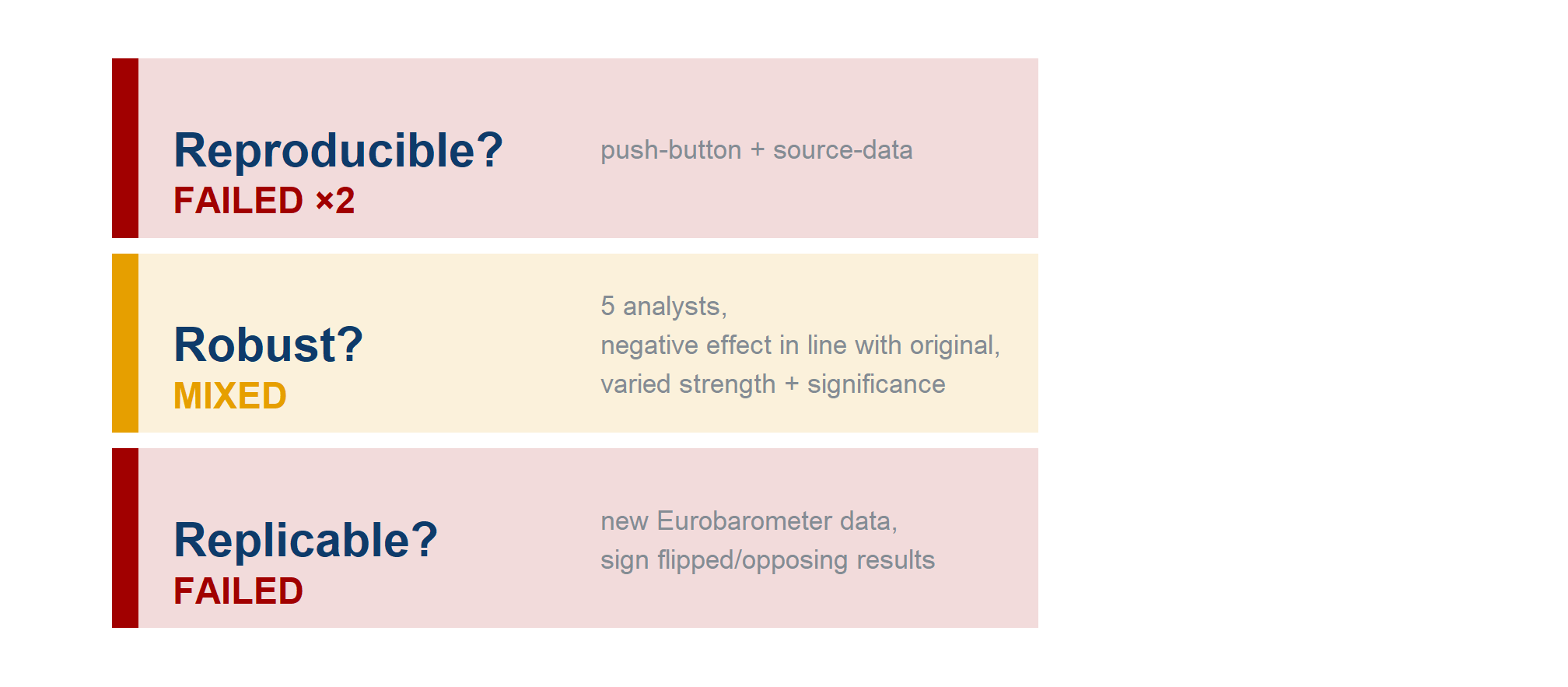
• Code: push-button reproduction failed

The reproduction attempt failed because the authors used file names that did not correspond with the names of the files available for download. Additionally 16 datasets are listed on the website as being used but the code references 18 files

• Source-data reproduction (rebuild from raw) – not reproduced: could neither extract nor re-calculate the original effect size

SCORE, the large research programme that Multi100 was part of, made two attempts to reproduce this paper, and each failed in its own way. [advance] In fairness to OA, there was no public archive with the paper, but OA did supply their two Stata do-files when asked; what OA could not share was the data, because the GESIS terms do not allow it. [advance] Even with that code in hand, the push-button reproduction failed, because the file names in the code did not correspond to the files you could actually download. The website listed sixteen datasets, and the code referenced eighteen files. The second attempt rebuilt the data from source, and could not recover the published effect size at all. So this claim entered the robustness study with two failed reproductions already behind it, of two different kinds.

Replication on new data

• Analysis One – the focal test on which SCORE evaluates the claim

  • 352,114 person-year observations in the analytic sample
  • b = 0.002, p = 0.046, se = 0.0008, t = 2.004

• Analysis Two – the still studying and no full-time education categories in the variable age when finished full-time education were not converted to missing values

  • 379,396 person-year observations in the analytic sample
  • b = 0.002, p = 0.017, se = 0.0007, t = 2.394

• Both give a positive coefficient for unemployment on cosmopolitan framing, significant at p-values of 0.05 or less, after controlling for selected predictors and for wave and country-level effects

• By the criteria used by SCORE, Analysis Two did not replicate the claim

osf.io/zt5y2/files/7efsw

The third R is replication, which takes the same question to new Eurobarometer data. Analysis One is the focal test on which SCORE evaluates the claim: three hundred and fifty-two thousand observations, and a coefficient for unemployment on cosmopolitan framing of plus point zero zero two, with a p-value of point zero four six. Analysis Two changes one coding decision. Respondents who were still studying, or who had no full-time education, stay in the sample instead of being set to missing, which takes it to three hundred and seventy-nine thousand, and the coefficient is again plus point zero zero two, now with a p-value of point zero one seven. Both estimates are positive and significant, so both point the opposite way from the claim on the card. And by the criteria used by SCORE, as the last line says, Analysis Two did not replicate the claim.

The three Rs on this paper

osf.io/h7432

Put the whole dossier together – every artefact here is public, and the link is on the slide. Reproduction failed twice, in two different ways. Robustness is mixed: five analysts, one sign, and sizes spanning two orders of magnitude. And replication, a preregistered study that took the same question to new Eurobarometer data with three hundred and fifty-two thousand observations, flipped the sign of the coefficient, which came out positive, just significant, and the wrong way round. So the one paper has received three different verdicts, one for each R. Across the whole SCORE programme the three verdicts barely predict one another, and this paper shows that pattern in a single case. The question worth asking of it is therefore in which sense it is reliable, since a plain yes or no does not fit. Of the three, the middle one is where five careful people disagreed with each other, and it is the only one that we can work on in the tasks. The rest of this part is about what they were disagreeing over.

The five free-phase analyses

Analyst	Free-phase predictor	Free-phase outcome	Estimator
018OL	GDP per capita (level)	positive framing, 7-item mean	crossed random intercepts
KEVF1	GDP growth	positive framing, 7-item sum	random intercepts
PRL47	log GDP + growth + crisis dummy	three positive-framing shares	three-level mixed
KQXUE	GDP growth and unemployment	cosmopolitan + utilitarian shares	country FE
C6HJR	GDP growth and unemployment	positive framing, 7-item share	two-way FE

• Five free analyses, five different questions – three of us never touched unemployment at all – and one shared recorded verdict: evidence for the claim
• The constrained phase then manufactured a common question; its five comparable answers span −0.006 to −0.45
• Conclusions can agree while estimates cannot even be compared – the two robustness questions that Multi100 was built to separate (Aczel et al. 2026)

Free-phase records: the public Multi100 dataset (osf.io/q5h2c), which contains only categorical verdicts and free-text reports. The models themselves were read from the analysts’ public code.

This table goes back to what the same five analysts did before they produced the estimates in the forest plot from earlier. Multi100 ran in two phases, and the table records the first one, months before the constrained task, when each analyst had complete freedom. GDP per capita for one analyst, GDP growth for another, a whole battery of GDP measures at three levels for a third – and three of the five of us never touched the unemployment rate at all. The outcomes differ too: a mean, a sum, a share, three separate shares. These are five different questions, in other words, and every one of us recorded the same verdict, evidence for the claim. [advance] Then the constrained task arrived and manufactured one common question, and the five comparable answers ran from minus point zero zero six to minus point four five. Conclusions agreed in words while the numbers disagreed by two orders of magnitude. That is five people working on one paper, and earlier you met twenty-nine teams working on one dataset.

Two studies to set beside our five

The disagreement among our five analysts follows a pattern that was described first, and at far greater scale, in two studies on which the rest of this part rests.

Silberzahn and colleagues (2018) – the red-card study from earlier, in which twenty-nine teams analysed one dataset to answer one question. Twenty of the twenty-nine intervals excluded 1, and nine did not.

Auspurg and Brüderl (2021) went back through all twenty-nine of those analyses and asked a question that the original had not: what was each team actually trying to measure?

The first establishes that careful people disagree, and the second explains why.

Silberzahn et al. (2018); Auspurg and Brüderl (2021)

Before we go further into our own case, I want to put two studies beside it, and one of them you have already met. [advance] Silberzahn and colleagues, the red-card study from earlier: twenty-nine teams, one dataset, one question, twenty intervals excluding one and nine not. There are all twenty-nine again, flattened onto a single line so that you can take in their spread at a glance. That study establishes that careful people disagree. [advance] The second one is new, and the rest of this part depends on it. Auspurg and Brüderl, twenty twenty-one, went back through all twenty-nine of those pipelines and asked something that the original had not thought to ask: what was each team actually trying to measure? [advance] So one study shows the disagreement, and the other explains it. Let me take the second one properly.

Four estimands in the red-card study

Auspurg & Brüderl re-read the 29 analyses and found four different estimands:

descriptive association · discrimination net of mediators · variance-maximising · exploratory

The dispersion came largely from a multiverse of questions, rather than from a multiverse of analyses.

Auspurg and Brüderl (2021)

Auspurg and Brüderl found that the twenty-nine teams had been answering four different questions. [advance] Some estimated the plain descriptive association. Some went after discrimination proper – the effect net of everything that legitimately explains red cards. Some built models tuned to explain variance, and some were frankly exploring. [advance] With four different questions in play, the answers were bound to differ. That reframes the crisis quite a bit, because much of what looks like analytical instability is unstated disagreement about what is being estimated.

Red-card estimates with and without a fixed estimand

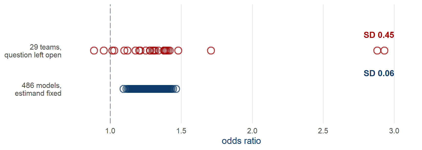
• Fix the question, derive the model space from a DAG, and run all 486 justifiable models: the SD falls from 0.45 to 0.06
• The 0.45 in the top row comes mostly from two analyses, the outliers beside a tight cluster

Auspurg and Brüderl (2021). Top row: the 29 published estimates. Bottom row: drawn to their reported median (1.28) and SD (0.06) – the 486 values are not published.

Auspurg and Brüderl then fixed one estimand – discrimination, properly defined – used a causal graph to derive every model specification consistent with it, four hundred and eighty-six of them, and ran the lot. The standard deviation falls from point four five among the twenty-nine teams to point zero six with the question fixed. The top row there is the twenty-nine published estimates themselves, and only the bottom row is drawn to the reported median and standard deviation, because those four hundred and eighty-six values were never published. The spread in the top row comes from a tight cluster and two outliers, which is why its standard deviation is about two and a half times what the cluster alone would give you, and with the question fixed even those two disappear. What we take from the study is the procedure that this course follows: a precise question, assumptions drawn out explicitly, then a whole multiverse rather than one path, then sensitivity analysis. [advance]

Under-specified research questions

Auspurg and Brüderl put the question in their title: has the credibility of the social sciences been credibly destroyed?

If the twenty-nine teams answered four different questions, most of their disagreement is not evidence that analysis is unreliable.

It is evidence that the question was under-specified – an ordinary, fixable defect.

Read this way, the many-analyst literature is a diagnosis of vague research questions rather than a verdict on social science.

This reading is more optimistic, and also more demanding, because it places the problem with whoever writes the question.

Auspurg and Brüderl (2021)

Now, this diagnosis has a consequence that goes well beyond the red-card study, and Auspurg and Brüderl put it in their title: has the credibility of the social sciences been credibly destroyed? If the twenty-nine teams were in fact answering four different questions, then most of their disagreement is not evidence that data analysis is unreliable. It is evidence that the question they were handed was under-specified, and that is an ordinary, fixable defect of research design. Read that way, the whole many-analyst literature stops being a verdict on the field and becomes a diagnosis of vague research questions. I find that a considerably more optimistic reading. It is also a more demanding one, because it takes the problem away from statistics, where you could hope a better estimator would save you, and puts it back on whoever writes the question, which in the tasks ahead means you.

Theoretical and empirical estimands

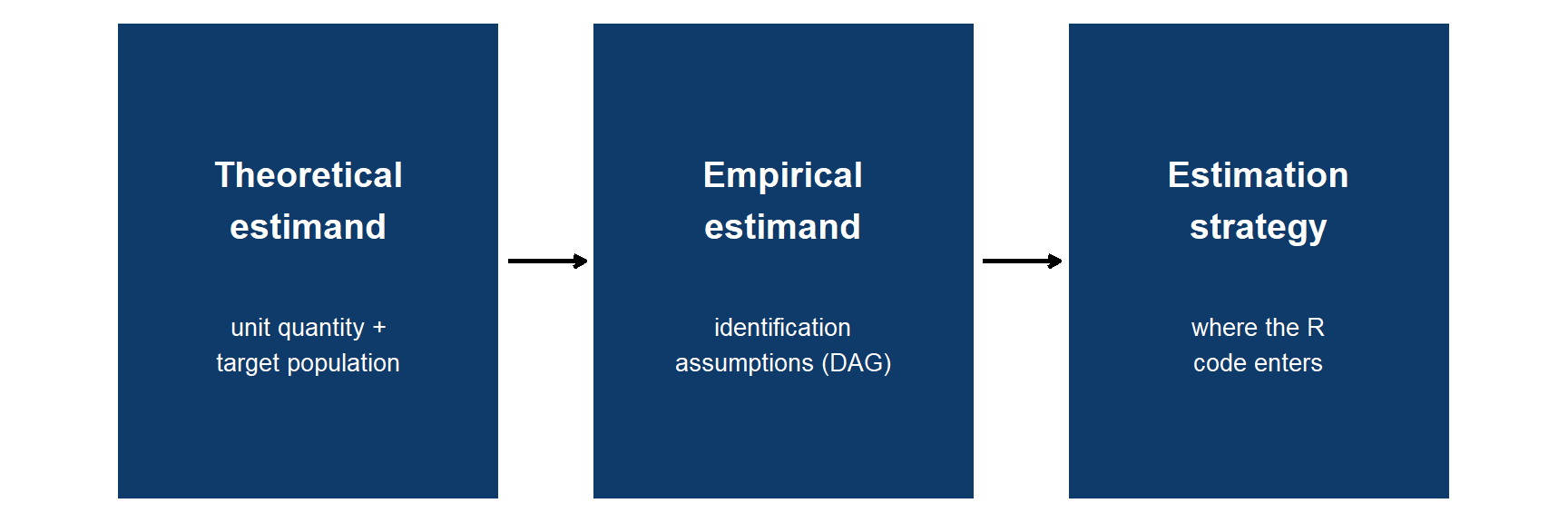
• The theoretical estimand is stated outside any model – before R opens

Lundberg et al. (2021).

Our five analysts and the twenty-nine red-card teams were all handed a question in words, and none of them was told exactly which quantity would answer it. Lundberg and colleagues call that quantity the estimand, and the title of their paper asks for it directly: What is your estimand? They split the answer into three steps. First, the theoretical estimand: a unit-specific quantity and a target population, stated in plain words, before any model exists. Second, the empirical estimand, which is what in the observable data corresponds to that quantity – and making that link forces your identification assumptions into the open, which is the job of the causal graph. Only third comes estimation, where R finally opens. When they audited a full year of papers in a top sociology journal, the unit quantity was clearly stated in five out of thirty-two. By their standard, every quantitative study must be able to answer that question before R opens.

Confounders, mediators and colliders

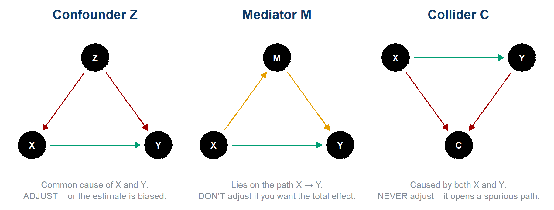
X = predictor, Y = outcome. Green = the causal effect you want; coloured = the path you must reason about.

The causal graph is the second of those three steps, and these three small graphs cover all the graph theory that the tasks need. In every panel the green arrow is the same thing, the effect of X on Y that you are actually after. What changes is the coloured structure around it. A confounder is a common cause of your predictor and your outcome – that red fork is a back-door path, and if you leave it open you are biased, so you adjust to close it. A mediator lies on the causal path between them. The amber path is real and part of the total effect, so if the total effect is what you want you do not adjust for it, or you remove part of the very thing you are measuring. And a collider is caused by both sides – those edges are harmless until you condition on the collider, which opens a spurious path that was not there before. So the rulebook is short: adjust confounders, leave mediators alone for total effects, and never condition on a collider. The next four slides add a little depth to those three rules before you use them.

Causal stories behind a correlation

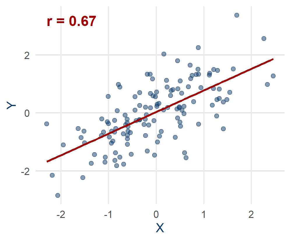
The same slope fits four different stories:

• X really causes Y – the slope is the effect

• a common cause inflates it – confounding

• the sample itself is selected – collider / selection

• Y causes X (reverse causation), or it is chance

The data look identical in all four. Only an assumption about how the data arose can tell them apart, and a DAG is where you write that assumption down.

D’Agostino McGowan et al. (2024); Keele et al. (2020). Scatter simulated for illustration.

The scatter here has a strong correlation, an r of about nought point six. Before you reach for a model, consider that this single number is consistent with at least four different stories. Maybe X really does cause Y, and the slope is the effect. Maybe a common cause is inflating it. Maybe we are quietly looking at a selected sample, and the association is an artefact of who got in. Maybe Y causes X, or it is simply chance. Nothing in the data can decide between these, because the scatter looks identical in every case. Only a claim about how the data were generated can do that. A DAG is where you write that claim down, and that is why we draw one before we fit anything.

Reading a DAG: open and closed paths

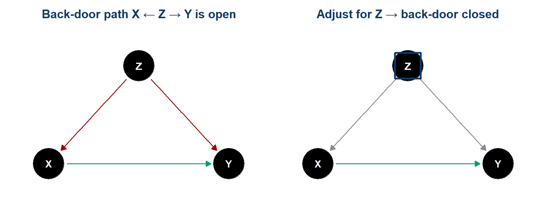
Association flows along every open path, not only along the causal arrow. A fork or a chain is open until you adjust for the variable in its middle. A collider is the reverse: shut by default, and opened when you adjust for it.

• Back-door criterion: close every path that enters X from behind, keep the causal X → Y path open
• Only an adjustment set that does this supports a causal reading

Hernán and Robins (2020); Huntington-Klein (2021).

A DAG is read through its paths. Association flows along every open path between X and Y, not only down the causal arrow. So the job is to work out which paths are open and shut the ones you do not want. Two rules do all the work. A path through a fork or a chain is open, and you close it by adjusting the variable in the middle – that is the red back-door fork on the left. A path through a collider is the opposite. It is shut by default, and you open it by adjusting. The back-door criterion puts the two rules together: close every path that sneaks into X from behind, and leave the causal X-to-Y path alone. Only an adjustment set that does that gives you an estimate you are allowed to read as causal.

Total effect or direct effect

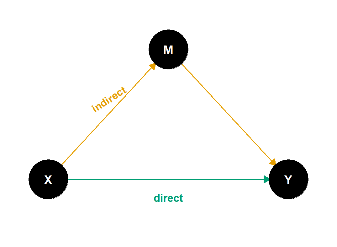
• Total = direct (green) + indirect (amber)
• Adjust for the mediator M → you estimate the direct effect only – a different estimand
• Control for everything can switch you to an estimand you never chose
• Table 2 fallacy: the other coefficients in your model are not all causal effects

Keele et al. (2020); D’Agostino McGowan et al. (2024).

Suppose M lies between your predictor and your outcome. The total effect is the green arrow plus the amber route through M. The direct effect is just the green arrow. These are different numbers and different questions – and which one you get depends entirely on whether you put M in the model. Drop a mediator in as just another control and you have silently switched to the direct effect without telling anyone, including yourself. This is why control for everything is bad advice. And it has a famous corollary, the Table 2 fallacy. When you print a regression table, usually only one coefficient has a clean causal reading. The coefficients on the control variables are not little causal effects of their own.

Selection and feedback

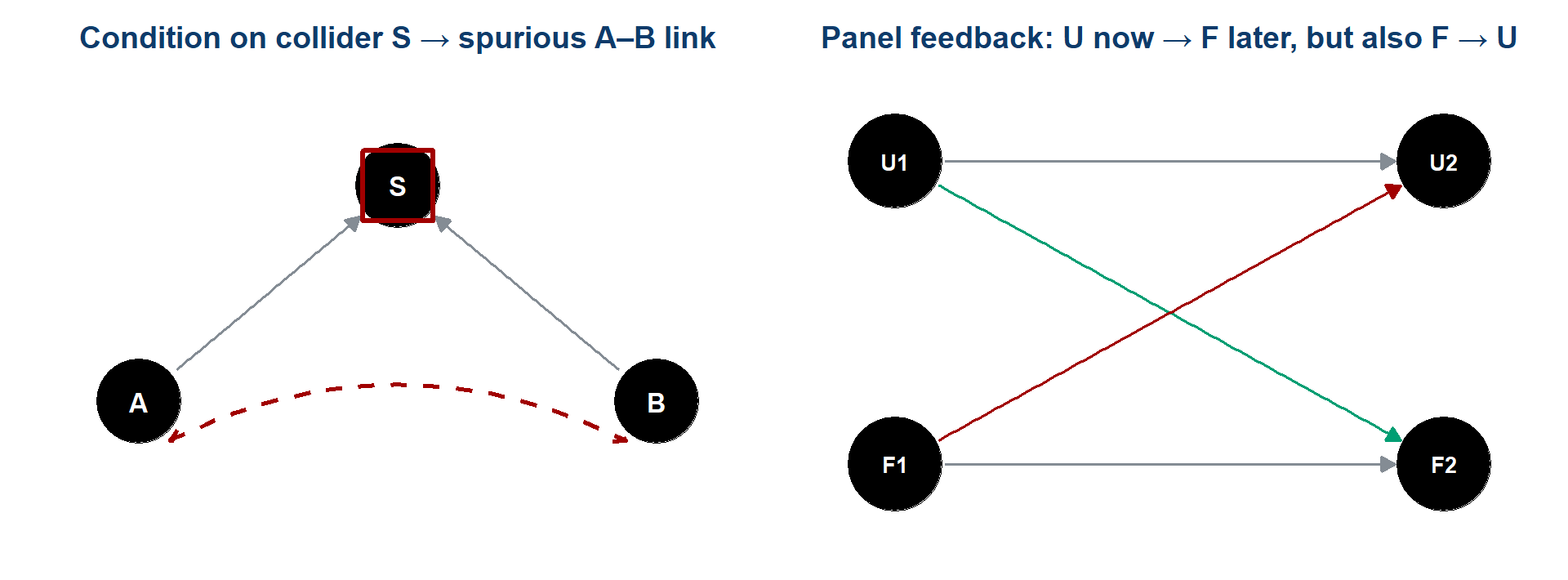
• Selection / collider bias – conditioning, or merely sampling, on a common effect manufactures an association that was never there (much of the early COVID risk-factor literature)
• Reverse causation & feedback – in a panel, today’s outcome can move tomorrow’s predictor; two-way fixed effects absorb stable country traits and common-year shocks, not time-varying feedback (U = unemployment, F = framing)

Griffith et al. (2020); Cole et al. (2010); Leszczensky and Wolbring (2022).

Two last ways a relationship can be spurious, and both of them apply to our case. The first is selection, or collider bias. If you condition on – or merely sample on – something that both your variables cause, you manufacture a correlation out of nothing. A lot of the early COVID risk-factor findings were of this kind, drawn from people who had been tested, which is a selected group. The second is reverse causation and feedback. Our data are a panel, and in a panel today’s outcome can feed tomorrow’s predictor. Two-way fixed effects, the baseline design for our own claim, soak up stable differences between countries and shocks common to a year. They do not, on their own, fix a time-varying confounder or a feedback loop. Keep that in mind when we build the graph for our own paper.

Revenons à nos moutons

The expected change in [unit quantity] among [target population] for a 1-percentage-point difference in unemployment, holding [assumptions] fixed.

• Unit quantity – a person’s cosmopolitan framing, or a country-year mean?
• Target population – which countries, which years?

In chat, now: your one-sentence estimand for the claim. Type it, hold it, send on go.

Back to our own paper, then, with the template from Lundberg and colleagues in hand, and this one is a chat exercise. Write the statement on the slide with the brackets filled in: your one-sentence estimand for the claim. Type it, hold it, send when I say go. [go; read three or four aloud.] Look at the spread in the chat – some of you wrote about a person’s framing, some about a country-year average, some named different years. None of those are wrong. They are different questions, with different confounding stories, and the coefficient means something different in each. That spread, in a class that has just followed the same slides, is the same kind of disagreement that the five free-phase analyses of our paper showed. Keep your statement, because it goes into your preregistration in Task 5, and when we reach the menu of choices you will also see what the choice of unit did to the estimates of the five analysts.

Causal identification in this design

Observational panel · 27 countries · no assignment mechanism · feedback between the variables · a decade of shared shocks.

Nothing in this design licenses unemployment causes a shift in EU framing.

So why draw a causal graph at all?

Because the graph still does three jobs that do not need identification:

• It says which association you are after – for instance the total effect, rather than whatever the software returns
• It tells you which variables belong in the model, and, just as usefully, which do not
• It makes your assumptions legible and arguable – a reader can disagree with an arrow, and that is a productive disagreement

The template you have just filled in speaks of an expected change in framing for a one-percentage-point difference in unemployment, which sounds causal, so it is worth being plain about what this design can deliver. This is an observational panel of twenty-seven countries. Nobody assigned unemployment to anyone. The variables plausibly feed back into each other over time, and the whole decade is shot through with shocks that hit everybody at once. Nothing in that design licenses the sentence unemployment causes a shift in EU framing. [advance] So why draw a causal graph at all? [advance] Because the graph does three jobs that do not need identification. It says which association you are actually after – the total effect, say, rather than whatever the software happens to return. It tells you which variables belong in your model, and just as usefully which do not. And it makes your assumptions explicit, so that a reader can disagree with a specific arrow, which is a more productive argument to have than one about a coefficient.

Publishing the estimand and the graph

The graph and the estimand are only worth anything if they are published where someone else can read them:

• in the paper itself
• before the model runs, not reconstructed afterwards
• with the limitations named by you before a reviewer finds them

In Task 5 you enter all of that in a block of the report in your workspace – the estimand, the graph-based justification, the one specification, and the rule for what would count as support – and you do it before you run the model.

The technical name for that is preregistration, and it fixes the question before anyone knows the result.

One more step follows from this, and it is where the tasks are heading. A graph you drew and did not publish is worth almost nothing. It has to be written down in the paper, where someone else can read it. It has to be written before the model runs, not reconstructed afterwards once you know which way the coefficient went, because a graph drawn after the fact will very reliably justify the result you already have. And you have to name the limitations yourself, before a reviewer finds them. [advance] In Task 5 you will enter all of that in a block of the report in your workspace: your estimand, your graph-based justification, the one specification you will run, and your rule for what would count as support – and you will do it before you run the model. [advance] The technical name for that is preregistration.

The EU-frames DAG, half built

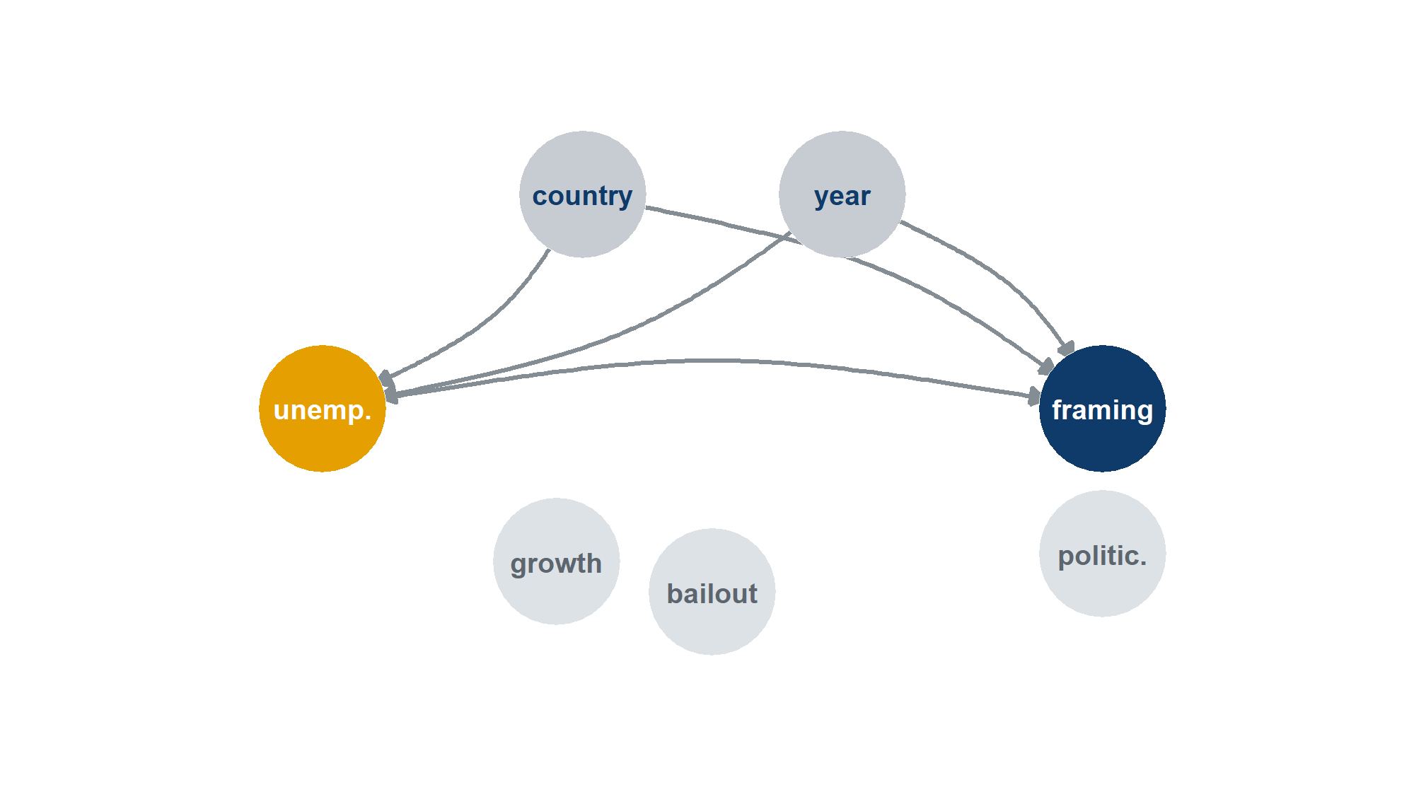
The same graph in R. Every arrow is a formula, read outcome-first – so a # takes an arrow out and the code still runs:

dagify(
  framing ~ unemployment,
  framing ~ country + year,
  unemployment ~ country + year,
  # framing ~ growth,        # uncomment the
  # unemployment ~ growth,   # arrows you believe
  exposure = "unemployment", outcome = "framing"
) |> adjustmentSets()

• Drawn: the path of interest and two confounders, country and year, which two-way fixed effects adjust for
• Not yet wired: growth (confounder?) · bailout (mediator?) · politicisation (mediator?)
• Your part: add the edges you believe, then run adjustmentSets()

This is the graph that you will finish yourselves. The solid part is what we are committing to: unemployment to framing is the path of interest, and country and year are the two confounders – stable national traits on one side, EU-wide shocks in a given year on the other. Run adjustmentSets() on this graph and it returns country and year, which is what a two-way fixed-effects model absorbs. So the graph and the baseline model make the same claim, once as a picture and once as a regression. The three pale nodes are yours to wire up, and they are genuine decisions. Is GDP growth a time-varying confounder that fixed effects cannot reach – a slump that raises unemployment and sours sentiment in the same year? Is the bailout a mediator, in which case you leave it alone if you want the total effect? Multi100 told us to disregard politicisation – was that defensible? The code beside the picture is the same graph written as R formulas, one arrow to a line, so wiring a node up means uncommenting the line you believe and running it again to see what the adjustment set has become. You do that in Hands-on 2, and the adjustment set you settle on there decides the model that you carry into the menu and into your preregistration.

Hands-on 2 – The panel, the estimand and the causal graph

Task 2 has three pieces:

1. Look at the data. 270 rows, 27 countries, 10 years. Run the country panel plot and find the ones that move
2. Write the estimand in words. The template gives you the unit quantity, the target population, the aggregation – fill in each for this claim
3. Wire up the DAG. Take the # off the arrows you are willing to defend, rerun adjustmentSets(), and check which adjustment set it now returns

Two sentences for your notes: what do two-way fixed effects adjust for, and what can they not fix?

Whatever you decide here becomes your starting point on the menu in Task 4, and the justification you preregister in Task 5.

Your turn, and this is the piece that people tell me afterwards changed how they work. Three things. First, look at the data – twenty-seven small panels, and find the countries that move sharply, because that is the variation that your model will use. Second, write the estimand in words using the template on the page: the unit-specific quantity, the population you want it over, and how you are averaging. Write it for this claim specifically, because the value of the exercise comes from having to be precise. Third, the graph. Take the hash off the arrows you actually believe, rerun, and look at what adjustmentSets gives back. If you add growth as a confounder, the adjustment set will include something that the two-way model cannot deliver. That is a real finding about the design, so do not go hunting for a bug in your code. Then those two sentences for your notes. [state the time] Shout in chat if you get stuck.

Lunch

An hour – the return time is in the chat · lunchtime browsing, if you like: the specification menu

Lunch – a full hour, and the return time is in the chat. If you want a head start on the afternoon, the specification menu page is worth five minutes with a sandwich: it is the list of choices you will pick from when you become the sixth analyst for real. See you back here.

DAY 2 · PART 2 – Reproduction and exploration

Day 2 · Part 2 · session 3

Part two of the day: the reproduction to the third decimal, then the menu and a run of exploration. The methodological tutorial waits for tomorrow, when there is time for it.

Task 2 of Multi100

Focus on the Cosmopolitan dimension for EU framing and on the unemployment rate as the independent variable; disregard contextual variables.

Three instructions. Everything else – estimator, sample, weighting, functional form, how you build the scale – was left to us.

Multi100 was designed to fix just enough to make the numbers comparable and to leave the rest free, so that what remained would be a measurement of analytical variability itself.

Here, word for word, is what Multi100 asked of us in its second task. Focus on the cosmopolitan dimension as the outcome, use the unemployment rate as the independent variable, and disregard the contextual variables. Three instructions – that is the whole brief. Everything else was left open: which estimator, which sample, whether to weight, what functional form, and even how to build the cosmopolitan scale out of the underlying items. And that is how the design was meant to work. Multi100 fixed just enough to make five numbers comparable and left the rest free, so that what remained would be a measurement of analytical variability itself rather than of anything about the paper. It follows that everything they left open is a place where five competent people could legitimately part company, and they did.

What those three instructions assume

• The cosmopolitan dimension assumes that the five items form one scale, and that the summary used in the paper, each respondent’s share of mentions, is the right one. A mean, a sum, or a factor score would all be defensible
• The unemployment rate assumes that the claim is about unemployment. The abstract of the paper says poor economic performances – which also names GDP growth
• Disregard contextual variables removes the country-level controls. That makes results comparable across analysts and gives up any defence against a time-varying confounder

None of these is wrong. Each one is a decision, made for you, that a different study could reasonably have made differently.

Now take those three instructions apart, because each rests on an assumption. The cosmopolitan dimension takes for granted that the five items – peace, democracy, freedom of movement, cultural diversity, a stronger voice in the world – form one scale, and that the summary used in the paper, each respondent’s share of mentions, is the right one. A mean would be defensible. So would a sum, or a factor score. The unemployment rate assumes that the claim is about unemployment, but the abstract of the paper says poor economic performances, which just as clearly names GDP growth – and in the first Multi100 task, where we were free to choose, three of the five of us used a GDP measure rather than unemployment. And disregard contextual variables strips out the country-level controls, which gives you comparability across analysts and gives up any defence against a confounder that varies over time. None of these is wrong. Each is a decision, made for you, that another study could reasonably have made differently.

The EU-frames panel

EUframes_cy.csv – 270 rows, one per country-year · 27 countries · 2004–2013

Column	What it is
cntry, year	the cell
mcosmo	mean cosmopolitan framing in that country-year, 0–1
mutil, mcomm, mlib	the other three framing scales
mpos, mneg	the two composites – all positive items, all negative items
unemp, growth	national unemployment rate and GDP growth
n_cy	how many survey respondents are behind the cell
bailout	1 if an EU/IMF assistance programme was running

n_cy is the interesting one: cells are built from very different numbers of people, which is why weighting is a live choice on the menu.

Here is the panel that you looked at in Hands-on 2, now column by column, because everything from now on works from it. Two hundred and seventy rows, one per country-year, twenty-seven countries over ten years. Country and year identify the cell. Mcosmo is the mean cosmopolitan framing in that cell, on a nought-to-one scale, and the other framing scales sit beside it. Unemployment and growth are the national macro indicators. And then n underscore cy, which counts how many survey respondents are behind each cell – and that is the interesting column, because those counts differ a great deal between cells. A country-year built from two thousand respondents and one built from five hundred are not equally precise, which is why whether to weight by n is a live choice on the specification menu. It is the one data file that you will load yourself.

Analyst no. 6

• Aim 1: reproduce analyst C6HJR’s constrained result

• What Multi100 asked: focus on the cosmopolitan dimension and on the unemployment rate; disregard the contextual variables

• What I submitted: a two-way fixed-effects model, mcosmo ~ unemp_c | cntry + year

• What Multi100 recorded: t ≈ −3.80 (df = 233, N = 270, partial r ≈ −0.242)

So here is your first job as the sixth analyst, and it is the same job I had. Multi100 asked for the cosmopolitan dimension, the unemployment rate, and no contextual variables. What I submitted was a two-way fixed-effects model – cosmopolitan framing on centred unemployment, with country and year absorbed – and what Multi100 recorded for me is a t of minus three point eight zero, on two hundred and thirty-three degrees of freedom, which standardises to a partial correlation of minus point two four. Now, you have my code. You have my data. The whole of reproducibility is the question of whether that is enough for you to get my number back. Let us find out.

Hands-on 3 – Reproducing the recorded result

• Task 3 in your workspace or in the browser lab – the constrained specification: outcome mcosmo, unemployment centred, country and year fixed effects
• The data are one file, EUframes_cy.csv, loaded as the object euframes
• In the working script the model is written out for you to run; the browser lab version has gaps to fill, with two hints and a full solution

Target: t = −3.804 – the value recorded for analyst C6HJR in the Multi100 dataset. When you have it, type your t in chat and hold it until I say go.

Now you work. Open the working script in your workspace and go to Task three. The code is written out there: it centres the unemployment rate on its grand mean, then fits the two-way fixed-effects model with fixest, so read it line by line as you run it. If you have fallen back on the browser lab, Task three there is a fill-the-gaps cell, with two hints and a fully worked solution underneath, and using either is not cheating, because this task is about the number at the end rather than the typing. You should land on t equals minus three point eight zero four, which is the value recorded for me in the Multi100 dataset. When you have it, type the t into chat but do not send – when I say go, everyone sends at once. Twenty minutes. [wait for the numbers in chat]

Reproducibility and analytical choice

Thirty of you just got t = −3.804, to the third decimal. That is reproducibility, and it is the easy R.

You all ran the same code. The five Multi100 analysts each wrote their own and came back with five different answers.

None of them was careless. They made different choices, and the options that they chose from make up the menu.

Look at what just happened. Thirty people, thirty machines, one number, agreeing to the third decimal. That is reproducibility, and I want you to notice how cheap it was: you all ran the same code on the same file, so of course you got the same number. Reproducibility is the easy R, and it is the one that this paper failed. [pause] Now hold that against the Multi100 chart from earlier – five analysts of this same claim, five different answers, one of them not even significant. Not one of those five was careless. I have read all four of the others’ code, line by line, and they are competent, well-organised pipelines written by people who knew exactly what they were doing. So the spread is not a quality problem. It is a problem of choices, and the menu is the full list of choices that were available to us.

The specification menu

Axis	Options
Outcome	mcosmo · mutil · mcomm · mlib · mpos · mneg
Outcome family	gaussian · beta (logit link, for a bounded 0–1 scale)
Predictor	unemployment · GDP growth
Predictor form	raw · log (unemployment only – growth goes negative)
Copredictor	none · the other macro measure
Estimator	two-way FE · country FE · random effects · pooled OLS
Sample	all · 2004–2008 · 2009–2013 · no bailout countries · no Greece and Spain
Weights	none · n_cell · n_eff · pop

Eight of the fourteen axes. The other six – scoring rule, no-opinion handling, item set, cell weighting, published series and standard errors – are on the specification menu page, with copy-paste code for every option.

Two of these axes already varied in the red-card study, where the 29 teams split across four response distributions (outcome family) and four ways of handling non-independence (estimator).

Here is the menu, and everything that follows is built on it. Fourteen axes, eight of them on this slide, and every option on it is a choice that a competent analyst could defend in print. Which framing scale is your outcome. Whether you model a bounded nought-to-one scale with a linear model or with something built for proportions. Whether you measure economic performance by unemployment or by GDP growth. Whether you take the rate raw or logged. Whether the other macro measure goes in beside it. Which of four ways you handle the fact that observations are grouped in countries and in years. Which countries and which years you keep. And whether you weight each cell, and if so by how many people were interviewed in it, by its effective sample size or by the adult population that it stands for. The menu page has copy-paste code for every one of these, so nobody is writing R from a blank line. [advance] Two of these axes are not new to you. In the red-card study the twenty-nine teams already split four ways on the response distribution, which is our outcome family, and four ways on how to handle observations that are not independent, which is our estimator.

What Task 2 of Multi100 left open

The three instructions fixed the outcome dimension, the predictor and the contextual controls. Everything else stayed open – including one thing that few people think of as a choice:

The unit of analysis. Two of the five fitted models on individual respondents; three worked on aggregates. Task 2 never said which, and the wording did not imply one.

Their five answers all obeyed the three instructions and still ran from r = −0.006 to r = −0.45, so the freedom that remained was enough to produce the whole spread.

The choices that move an estimate most are usually made before any model is fitted.

So what did those three instructions actually pin down? The outcome dimension, the predictor, and the contextual controls. Everything else stayed open – including one thing that almost nobody thinks of as a methodological choice at all, which is the unit of analysis. Two of the five of us fitted models on individual respondents, hundreds of thousands of them. Three worked on aggregates. Task two never said which, and the wording did not imply one either way. And the consequence is on the next fragment: five answers, all obeying all three instructions, still running from minus point zero zero six to minus point four five. The freedom that remained after the constraints was more than enough to produce the whole spread. Hold on to that, because it generalises: the choices that move an estimate most are usually the ones made before a model is fitted at all.

Ground rules for the menu

In Hands-on 4 the rule is: change one axis, hold the other thirteen at baseline.

Baseline = the specification you reproduced in Hands-on 3: mcosmo · gaussian · unemployment · raw · no copredictor · two-way FE · all years · unweighted · share of mentions · standard measurement settings · conventional SEs.

Changing one axis at a time keeps the class chart readable. Every dot differs from a common baseline on exactly one axis, so when a dot moves you can say what moved it.

And one convention binds everyone: claim-alignment. The negative framings are reverse-coded, 1 − y, so that supports the claim reads as a negative sign whatever your outcome. Without it the class chart would straddle zero by construction and look like noise.

Two ground rules before you touch the menu. First, one deviation: in Hands-on 4 you change one axis and hold the other thirteen at the baseline, which is the specification you reproduced in the third hands-on – cosmopolitan outcome, gaussian, unemployment raw, no copredictor, two-way fixed effects, all years, unweighted, the answers scored as shares, the standard measurement settings and conventional standard errors. That sounds restrictive, but it is what makes the class chart readable. Every exploratory dot on the chart will differ from one common baseline on exactly one axis, so when a dot sits somewhere surprising we can say what put it there. Second, a convention that binds everybody: claim-alignment. If your outcome is one of the negative framings, it gets reverse-coded – one minus the scale – so that supporting the claim reads as a negative sign for every outcome that anyone picks. Without that, half the class would be above zero by construction and the chart would look like noise.

Hands-on 4 – Exploring the menu

Task 4 is exploratory. Try several specifications, look at what each one does, and get a feel for which axes move the estimate.

1. Start from the baseline you reproduced
2. Change one axis in try_spec() and read what happens to b, t and the partial r; my_experiments() lists every try
3. Do it again with a different axis. Three or four is plenty
4. Then rerun the one you can argue for best with try_spec(), so that it is your last try, and submit it with submit_exploration()

Your dot appears on the live Multiverse page within seconds, and we read the dots from the whole class once everyone has submitted.

This is not your preregistered analysis. You are allowed to look, change your mind and try again, which is why this phase has a name of its own.

Right. This is where you get your hands properly dirty, and I want to be explicit about what kind of activity it is, because it differs from the preregistered analysis that comes later. Task four is exploration. Start from the baseline you reproduced. Change one axis with try underscore spec, and look at what happens to the coefficient, the t and the partial r. Every try is logged, and my underscore experiments lists them for you. Then do it again with a different axis – three or four goes is plenty. Then rerun whichever one you can argue for best with try underscore spec, so that it is your last try, and submit it with submit underscore exploration, which sends whatever you tried last. Your dot appears on the live multiverse page within seconds. Once everyone has submitted, we read what the class built. The second fragment matters: this is not your preregistered analysis. Here you are allowed to look, change your mind and try again. Most published work never says that such a phase took place, which is why this one has a name of its own.

Break

30 minutes – the return time is in the chat · leave the Multiverse page open

Break – thirty minutes, and the return time is in the chat. Leave the Multiverse page open in a tab, because the class chart on it is where your results go, and we read it together in the next part. If anything has not worked so far – a workspace that will not run, or a submission that has not reached the chart – flag it in chat and we will sort it out over the break, so that everybody gets a dot.

DAY 2 · PART 3 – Multiverse and preregistration

Day 2 · Part 3 · session 4

Part three of the day: the class chart, which fork accounted for the largest share of the variation, your percentile, what the curve leaves out, and the preregistration. The multiverse tutorial and the inference material wait for tomorrow.

Your own small multiverse

You ran three or four specifications, all defensible, and watched the estimate move.

Nothing about that is unusual. Every analysis you have ever published came from a space like that – you reported one point from it.

The multiverse idea is the proposal that the space is itself a finding, and that showing one point without it is a form of incomplete reporting.

In Task 4 you ran three or four specifications, every one of them defensible, and you watched the estimate move around. Now – nothing about that is unusual or improper. I want to say that clearly, because there is a slightly accusatory tone in some of this literature that I do not think is deserved. Every analysis any of us has ever published came from a space like the one you were wandering around in. The difference is that we reported one point from it and did not mention the rest, mostly because it did not occur to us that the rest was reportable. So the multiverse idea is a proposal about reporting, and not an accusation. The space itself is a finding, and showing one point from it without the space around it is a form of incomplete reporting.

The class multiverse

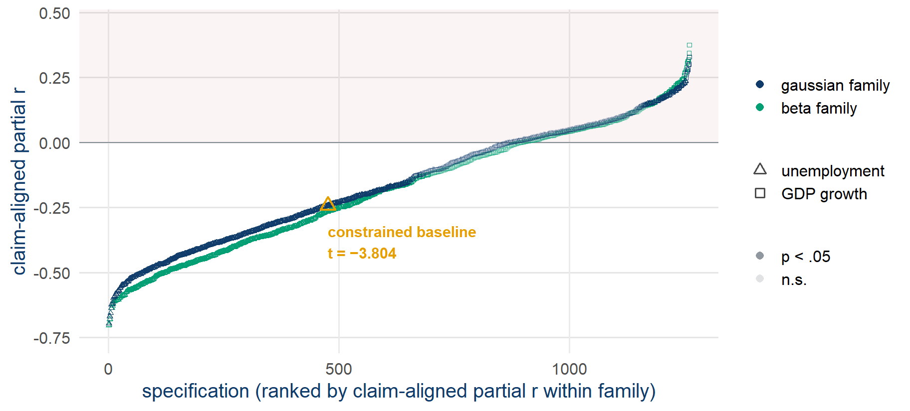
• The universe of 2,520 specifications: the Multi100 grid of 840 (blue unemployment triangles) plus the outcome-family and predictor axes, all at the standard measurement settings
• The grid of 840: 68.7% claim-consistent direction · 63.9% significant · claim-aligned partial r from −0.70 to +0.24

Pre-computed over the specification menu (data/spec_grid_full.csv), claim-aligned – negative framings reverse-coded and growth predictors sign-flipped, the convention that the preregistration block in Task 5 records (claim_align = TRUE).

This is the space of specifications – the same chart on which the Multiverse page has been drawing your dots. The grid of 840 with the outcome-family and predictor axes added, all run at the standard measurement settings: two and a half thousand models, each one a point, ranked by partial correlation within its family. Blue is the gaussian family, and the eight hundred and forty of the Multi100 menu are its unemployment triangles. Green is the beta twin of each, and the squares are the models that use GDP growth as the claim predictor. Everything is claim-aligned, the same convention you applied in your own code: negative framings reverse-coded, growth sign-flipped, so below zero means supports the claim, whichever outcome and whichever predictor. Faded points miss significance. On those eight hundred and forty, about two thirds sit below the line and about two thirds are significant. The orange triangle is the baseline we all reproduced. Support reaches minus point seven, while nothing climbs past plus point four – and the strongest wrong-sign results are growth squares. Right. Where did the class results fall? Did anyone end up above the line? Lose significance? Which choice moved your estimate most?

The published results on the curve

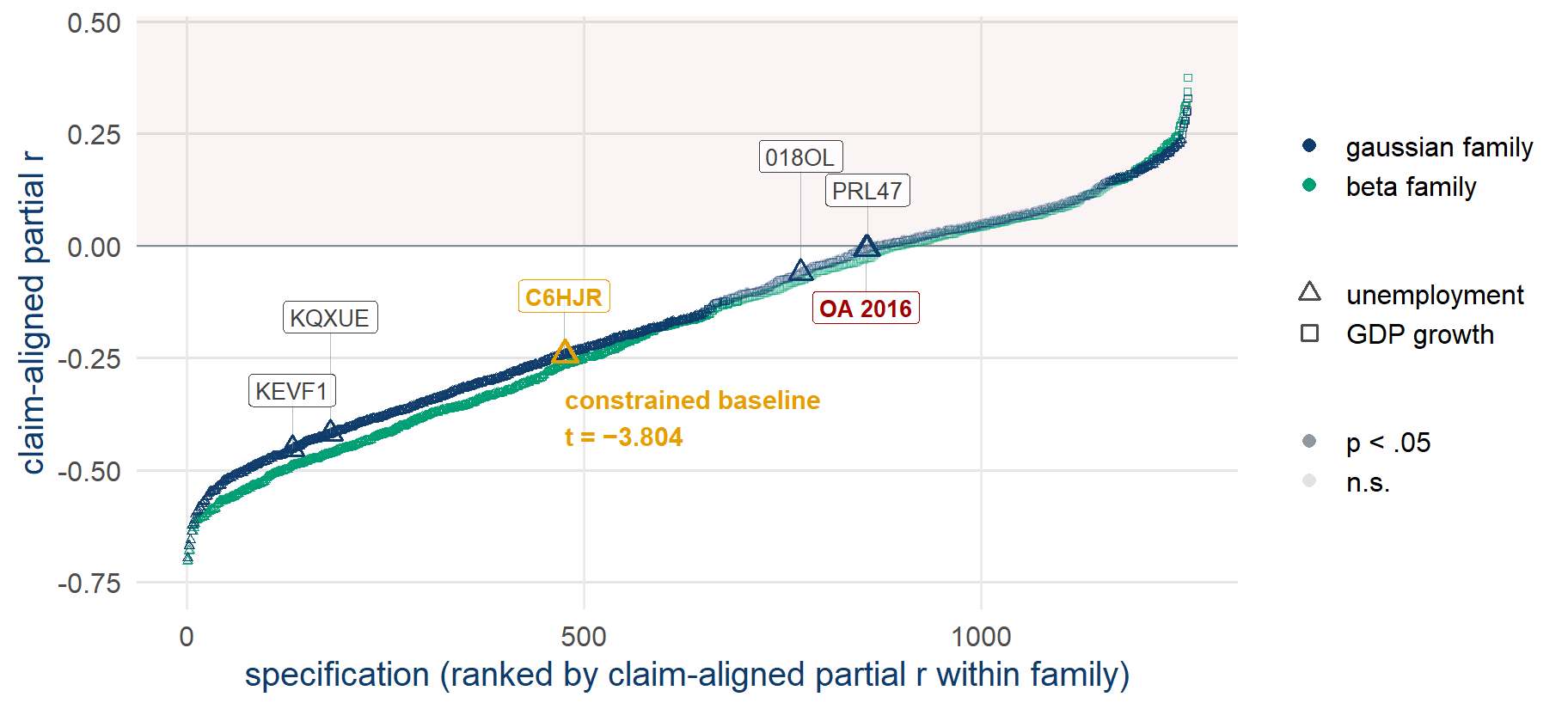
Your own dots are on the live Multiverse page, drawn on this same chart

submit_exploration() in Task 4 and report_result() in Task 5 each give you a one-click link to the Google Form; results appear on the Multiverse page.

Same chart – nothing moved – with the five Multi100 analysts dropped onto the curve where each recorded result falls, me in orange. And one more tag, in red: the original author’s own published result, converted to this axis the same way. A person-level t of minus four, read against a third of a million respondents, falls just beside PRL47’s near-zero triangle. That placement illustrates the degrees-of-freedom argument from the statistical methods module. The five published reanalyses are themselves draws from the wider space of defensible analyses, two of them from person-level models that this menu does not contain, and that is what I find most useful in the picture. Nobody was wrong; each of us made a different set of defensible choices. Your own dots have been on the live Multiverse page since you submitted them in Task 4, so keep it open next to this chart and find yourself. The conversion that try_spec and submit_exploration did for you in Task 4 – turning your b and t into the partial correlation, computed the way that Multi100 computed it – is what lets a Stata pooled model, an R fixed-effects model and your submission all be placed on the same axis.

A bet on the six axes

Six axes: outcome · predictor form · estimator · copredictor · sample · weights

Which axis moves the estimates most across all 840 specifications?

Type your guess – hold it – send on go.

Before I show you the answer, commit to a guess. You have made these choices yourselves in the hands-on, so you have instincts now. Of the six axes of the grid of 840, which one moves the estimates most across the whole grid? Estimator is the popular pick, because fixed versus random effects is the favourite fight in methods seminars. Copredictors is another, since everyone worries about growth. Type your answer, hold it, and send on go. [go; scan the chat.] Interesting spread. Most classes bet on estimator or copredictors. Let’s see.

Fork importance

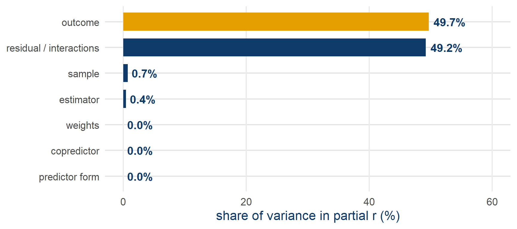
• Outcome operationalisation: 49.7% of specification variance · estimator + predictor form + copredictor + weights together: under 2%
• Computed on the grid as estimated – most of the outcome share is the polarity split between positive and negative framings, the split that the claim-aligned chart removes from display

Computed over the committed data/spec_grid.csv; imported as data/fork_importance.csv.

The outcome fork accounts for just under half of all the variation in the grid – forty-nine point seven per cent. And now look at the bottom of the chart. Estimator, predictor form, copredictor and weights are the axes we argue about in seminars, and together they account for under two per cent. The residual block is interactions, combinations that matter beyond any single axis. One caveat: this decomposition is computed on the grid as estimated, before claim-alignment, so most of the outcome share is the polarity split itself – positive framings falling, negative framings rising. That split is real variation in what the specifications estimate. The aligned chart removes it from the display, not from the decomposition. On the claim-aligned scale the ranking reverses. In my extended analysis of the same grid, the estimator then accounts for about fifty-eight per cent and the outcome about twelve, because once every framing points the same way, the gap between the pooled model and the other three estimators is the largest difference left. The to-weight-or-not debate barely moves the estimate on either scale. Whoever guessed outcome in the chat: take the point.

The five analysts in the grid

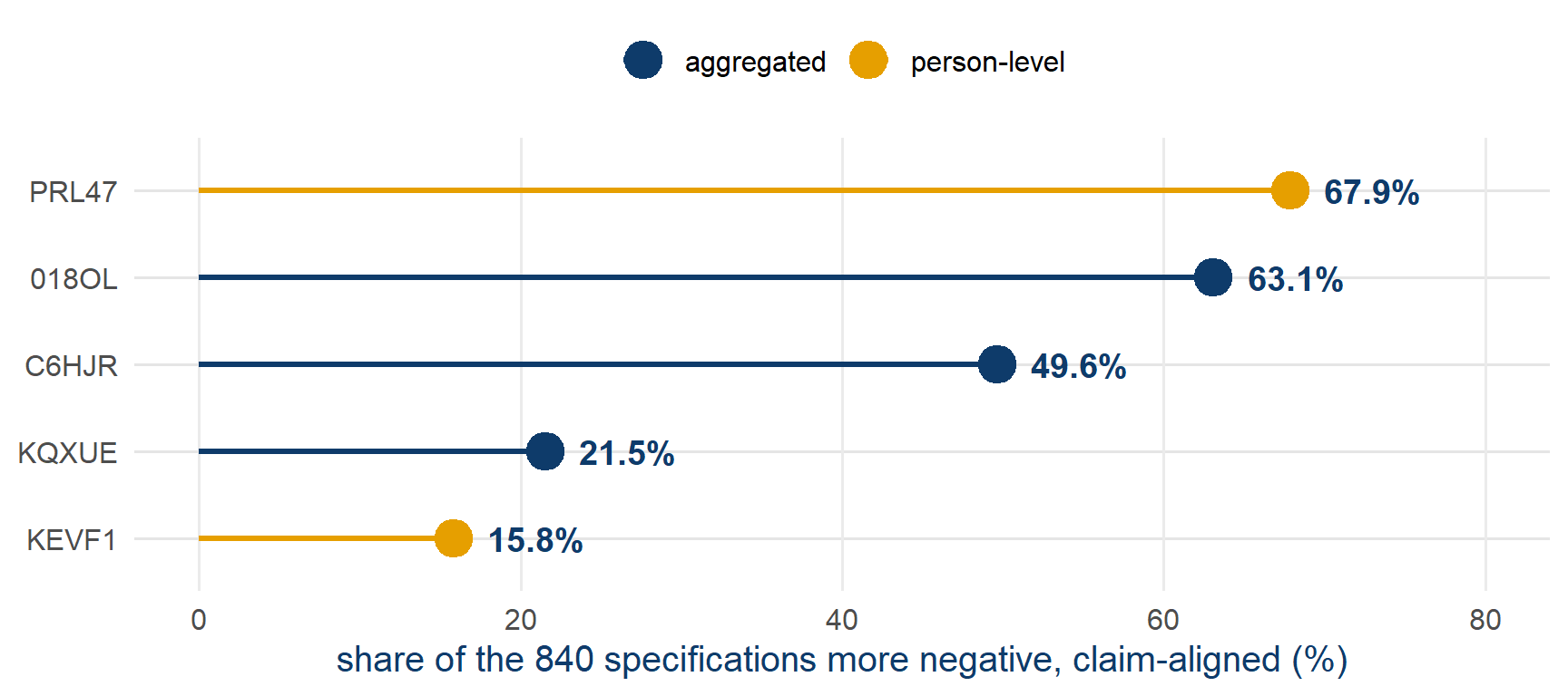
• The two person-level analysts are at the two extremes of the recorded range, so the unit of analysis and the metric matter more than the software or the estimator

Now put the five published analysts inside the same grid – for each one, the share of all eight hundred and forty claim-aligned specifications that come out more negative than their value. And look who is at the ends. KEVF1, the most strongly claim-supporting of the five at around the sixteenth percentile, and PRL47, the closest to the null at around the sixty-eighth – those two, at the opposite extremes, are the two analysts who worked at person level, on the third of a million respondents, rather than on aggregates. The three aggregate pipelines sit between them; my own constrained baseline falls almost exactly at the median of the grid. Five competent people end up scattered across half the curve because of the unit of analysis and the outcome metric, both decided before any model is fitted, rather than because of Stata against R or the choice of estimator.

Sign flips by estimator and sample

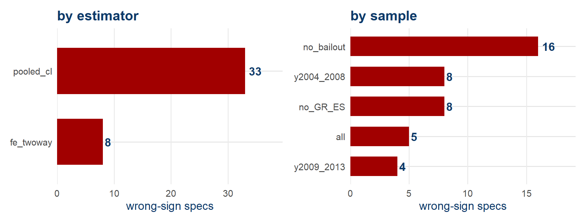
• In the cosmopolitan-only universe, the wrong-sign estimates concentrate in the pooled cluster-robust estimator and the bailout-excluding samples

The grid can also be read for where the sign flips occur. Take only the cosmopolitan-outcome specifications – the claim predicts a negative coefficient, so a positive estimate is a flip – and cross-tab the flips by axis. They are not scattered randomly. The estimator that absorbs no between-country differences at all – the pooled model with clustered errors – accounts for thirty-three of the forty-one, and the flips are also concentrated in the samples that exclude the bailout countries. In other words, when this claim flips sign, it flips for identifiable, diagnosable reasons: let the between-country comparison into the estimate, or remove the crisis countries, and the association goes. Taken apart like this, a specification curve lets you name the choices that produce its extremes, and the same grid can place any single result, your own included.

Your own percentile

• In the browser lab, rerun try_spec() with the choices you submitted in Task 4: its output includes your placement. Everyone uses the lab for this step, because the workspace does not print it
• The placement is the share of the 840 specifications more negative than yours, on the claim-aligned scale
• The same statistic that placed the five analysts, computed for you

Paste your percentile in chat – hold – send on go.

Your turn to be placed. Open the browser lab – everyone, because the workspace does not print this and the lab runs in any browser tab – and rerun try underscore spec with the choices you submitted. The placement line in its output is the same statistic that I computed for the five analysts: the share of the grid of 840 that is more negative than your value. Two or three minutes. Then paste your percentile in chat, hold it, send on go. [go] Look at the range in the chat – the class spans a good stretch of the curve, and every one of you can now say where you stand relative to eight hundred and forty defensible alternatives. That sentence – my estimate sits at the Nth percentile of the specification space – is a publishable way to report a robustness check, and you have just done it.

Critics of the multiverse

• Robustness is better assessed with a few thoughtful models than with billions of regressions (Auspurg 2025; answering Ganslmeier and Vlandas 2025) – only justified models targeting the same estimand belong in one curve. Our grid is a curated 840, and a decomposition by fork does the job that every critic endorses: it locates where the argument must happen
• There is only one correct analysis once the question is fully specified (Lakens et al. 2026) – your preregistered specification guards against cherry-picking, and their deeper point is that preregistering a choice does not yet make it justified, which is what the estimand and DAG work were for
• What’s a multiverse good for anyway? – reflection, persuasion, or inference, and each purpose needs a differently built universe (Rohrer et al. 2026). Ours was built for reflection, and how much more to read into it is the open debate

The book-length how-to: Young and Cumberworth (2025); the estimand diagnosis of the red-card study: Auspurg and Brüderl (2021).

The method you practised is the subject of a live debate, and you can now read that debate for yourself. Katrin Auspurg, who with Josef Brüderl traced the spread in the red-card study to teams answering different questions, answered a 3.6-billion-estimate study with the line at the top of this slide: only thoughtful, justified models belong in a curve. Our own grid is built mostly the way she recommends. It is a curated eight hundred and forty rather than an enumeration, and decomposing it by fork does the one job that every critic endorses, which is to show where the argument has to happen. Lakens and colleagues say that once the question is fixed, only one analysis implements it correctly. A preregistered specification guards against cherry-picking. Their deeper point, that preregistering a choice does not make it justified, is why the DAG comes before the preregistration. And Rohrer, Hullman and Gelman ask what a multiverse is for: reflection, persuasion, or inference, each needing a differently built set. Ours was built for reflection, and how much more can be read into it is the open question in the debate you have now joined. [advance]

The one-correct-analysis argument

The argument from Lakens and colleagues runs in four steps:

• A research question, fully specified, implies a quantity to be estimated
• That quantity, together with the design and the assumptions you are willing to make, implies one analysis that estimates it
• So a spread of results is not evidence of legitimate diversity. It is evidence that most of those specifications are wrong – they estimate something else
• On this reading, showing a wide curve is closer to an admission than to a robustness check

Take it back to the red cards. Twenty-nine teams modelled one count of red cards as linear, logistic or Poisson. Those are claims about how the outcome was generated, and they cannot all be right – so on this argument most of the spread is error.

Lakens et al. (2026)

The strongest objection to the multiverse approach comes from Lakens and colleagues, and I want to give it its full force. They argue that a research question, once fully specified, implies a quantity to be estimated. That quantity, together with your design and the assumptions you are prepared to make, implies one analysis that estimates it. From which it follows that a spread of results is evidence that most of those specifications are wrong, because they estimate something other than what you said you wanted, and not evidence of legitimate analytical diversity at all. And on that reading, publishing a wide specification curve is closer to an admission that you never specified your question than to a robustness check. That is an uncomfortable argument and I think it is largely right.

Identifying the one correct analysis

Grant the argument, and suppose that one correct analysis exists. Which one is it?

Getting there needs the estimand and the identification assumptions and agreement about the measurement – and on this claim, reasonable people disagree about all three.

So the curve complements the one-correct-analysis view: it is a map of the disagreement that remains, drawn because we cannot yet settle it.

And it points at what to argue about: on this claim, at the outcome, not at the estimator.

So let us grant the argument. Suppose one correct analysis does exist. The next question is which one it is, and how you would know. To get there you need the estimand, and the identification assumptions, and agreement about how the construct is measured – and on this claim reasonable people disagree about all three, as you found for yourselves in the hands-on tasks. So I read the curve as a companion to the one-correct-analysis view rather than a rival to it. It is a map of the disagreement that remains, drawn because we cannot yet settle it. Read that way it is useful, because it shows where the disagreement is. On this claim it is at the outcome – what EU framing means – and not at the estimator, which is where the seminar argument would have been.

What preregistration settles

It does settle

• That your specification was not chosen because of the result
• That your rule for what counts as support was fixed before you had a result
• That a reader can see what you intended, and what you changed

It does not settle

• Whether the specification was any good
• Whether it estimates the quantity that your question implies
• Whether the assumptions behind it hold

A badly reasoned analysis that is preregistered is still badly reasoned; the preregistration only adds a timestamp

That is why the estimand and the DAG came first today: preregistration protects a choice, and the causal reasoning is what justifies it.

So where does preregistration fit? It settles a specific and limited set of things, and the two columns matter equally. On the left: it settles that your specification was not chosen because of the result it gave, that your rule for what counts as support was fixed before you had a result to bend it around, and that a reader can see both what you intended and what you subsequently changed. Those are real guarantees and no other mechanism provides them. On the right, what it does not settle: whether the specification was any good, whether it estimates the quantity that your question implies, or whether its assumptions hold. A badly reasoned analysis that is preregistered is still badly reasoned, only now with a timestamp on it. That is why we did the estimand and the graph first. Preregistration protects a choice, and the causal reasoning is what justifies it.

Exploration and preregistration

• Aim 2: assess the robustness of the constrained result

• In Task 4 you explored: several specifications, tried in order to find out what they do. That was the right way to learn them

• In Task 5 you preregister one specification: it goes into the preregistration block of your report before it runs, with a reason that your DAG supports

• The code is identical. The difference is that one of these can be chosen because of its result and the other cannot

Earlier you reproduced my constrained result, and in Task 4 you explored – several specifications, tried in whatever order took your interest, in order to find out what they do. That was the right way to learn them, and I want to be clear that there was nothing improper about it. Now comes the other half. In Task 5 you preregister one specification: it goes into the preregistration block of your report before it runs, with a reason that your causal graph supports. The code for the two activities is identical. The difference is that one of them can be chosen because of the result it gave, and the other one cannot, and almost no published paper says which of the two it is reporting.

Hands-on 5 – The preregistration

1. Open the preregistration block in your report
2. Complete fields 1–5: the claim, the data-in-hand statement, your one specification, the one-sentence justification from your DAG, and your rule for what supports or undermines the claim
3. Render, or on the browser lab page copy the completed cell into your notes
4. Type declared in chat – then wait for the class

Nobody runs a model until everyone in the class has completed their preregistration block.

We preregister together, because a thing that the whole class does at once sticks in a way that an instruction does not. Open Task 5. Fill in the five fields: the claim, the data-in-hand statement, your one specification across the fourteen axes, the one-sentence justification that your graph gives you, and the rule – written now, before any result – for what would support the claim and what would undermine it. The data-in-hand statement is where you record what you already know about the data before you fix your specification. Render the report; the rendered file with its timestamp is the dated record of your preregistration, like the frozen snapshot that the OSF keeps of a registration. On the browser lab page, copy the completed cell into your notes. Then type declared in chat, and wait. [count them in aloud: eight declared… twelve…] Nobody runs anything until the whole class is in. And if the specification you choose is one that you already tried in Task 4, that is allowed, but say so in the block, because a specification whose result you have already seen is not preregistered in the strict sense.

Hands-on 5 – The preregistered run

• Task 5 – run the specification in your preregistration, and only that one
• report_result() prints a one-click link to the Google Form with your results already in it – click, submit
• Your dot joins the Multiverse page as a declared result (the chart’s name for a preregistered specification), beside the exploratory ones from Task 4

Compare the two waves. If the preregistered dots fall systematically to one side of the exploratory ones, it is worth discussing why.

Stuck? Chat STUCK · reload and rerun · second browser · follow my screen · last resort: the grid lookup on the menu page gives you the results for your specification by hand

Go. Run the specification in your preregistration, just that one, and when the numbers are in front of you call report underscore result: it prints a link to the Google Form with your values already filled in, one click and you have submitted. Your dot joins the chart as a declared result, which is the chart’s name for a preregistered one, and it appears beside the exploratory dots that the class submitted in Task 4. If the preregistered dots fall systematically to one side of the exploratory ones, that tells you something about what people chose to preregister once they had tried the alternatives, and it is worth a conversation. If anything misbehaves: type STUCK in chat and work down the ladder on the cheatsheet. And if your machine is truly finished for the day, the menu page shows you how to read the numbers for your specification straight off the published grid. Everybody gets a dot on the chart, no exceptions.

Two points from the literature

the common single-path analyses in social and behavioural research should not be simply assumed to be robust to alternative analyses (Aczel et al. 2026)

A blueprint: precise question → causal reasoning (DAG) → multiverse → sensitivity analysis (Auspurg and Brüderl 2021)

• Same-conclusion robustness and same-number robustness are different bars
• Justifiability is the criterion – choose with reasons, show the spread

The first point comes from the Multi100 paper: single-path analyses should not simply be assumed robust. And notice what preregistration did and did not do for you today. It protected your choice from being opportunistic, but it gave your preregistered dot no special status inside the curve. The preregistration made your one path defensible, and the grid showed that it was still one path among 840, so a report needs the preregistered path and the space around it together. From Auspurg and Brüderl comes the constructive recipe we followed – precise question, explicit assumptions, multiverse, sensitivity. And keep the two robustness standards apart in your own writing: same conclusion, which was seventy-four per cent in Multi100, and same number, which was thirty-four. When you claim robustness, say which one you mean.

The single analytical path

There is no privileged single analytical path – only justifiable ones, explored openly.

You made one justifiable choice today, preregistered it with its reason before running it, and placed it inside a multiverse.

codemoreh.github.io/applied-replication

Everything is open, and you can fork any of it.

There is no privileged single analytical path – only justifiable ones, explored openly. You have already done this once today: you made one defensible choice, you entered it and your reason in the preregistration block before running it, and you placed its result inside the space of alternatives. That habit transfers to any analysis you do, and the tooling, the estimand, the graph and the curve were all there to support it.

What you take with you

• Yours now: a rendered report with its preregistration block · an estimand statement and a causal graph that you wrote yourself · two dots on the class chart, one exploratory from Task 4 and one preregistered from Task 5
• Read: the three Nature 2026 papers (Miske et al. 2026; Aczel et al. 2026; Tyner et al. 2026) · the glossary (Nosek et al. 2025) · Auspurg and Brüderl (2021) · Lundberg et al. (2021) · Lakens et al. (2026) · Teney (2016)
• Explore: the sixteen companion modules (among them intro to R · Quarto documents · the statistics behind today · causal graphs · the multiverse debate · simulation · the individual level · repositories & preregistration · git & GitHub) · the Multi100 data · fixest & ggdag docs
• Keep going locally: the research-software and open-research teams at your university · a ReproducibiliTea journal club near you
• Everything is on the course site, and everything is open – fork any of it

You take home a rendered report with a preregistration block in it, an estimand statement and a causal graph that you wrote for a real published claim, and two dots on the class chart, one exploratory from Task 4 and one preregistered from Task 5. The website on screen has everything else – the readings, the data, the companion modules, the specification-curve reading, and the full SCORE dossier on the paper if you want to dig further. Two pointers for keeping the habit alive wherever you work: most universities have a research-software engineering team and an open-research or library data service that run training like today’s, and ReproducibiliTea journal clubs meet in dozens of cities – if there is not one near you, they will help you start one.

DAY 3 – The methods in depth

Day 3 · four sessions

Day three goes slowly through everything that yesterday took at speed. First the axes of the menu that set the question and the model, each shown doing something to an estimate. Then where the multiverse idea came from and what it is for, why hundreds of estimates are not hundreds of tests, and what a curve-level test would have to do. And then where a finished reanalysis is archived and registered. The companion modules fill the rest of the day – the graphs, the estimators output by output, weights, missing answers, simulation and version control.

The six framing scales

Methods tutorial · 12 slides · skip to Hands-on 4 →

Scale	Items	Claim predicts
mcosmo	peace · democracy · free movement · diversity · voice	negative
mutil	prosperity · social protection	negative
mcomm	unemployment · identity · crime · borders	positive
mlib	bureaucracy · waste of money	positive
mpos	all seven positive items	negative
mneg	all six negative items	positive

The claim says decrease positive dimensions – mpos is the more literal reading, mcosmo is what was instructed. Across all six scales, the choice of outcome accounts for roughly half the variance in the grid as estimated, most of it because positive and negative framings take opposite signs. The disagreement between mpos and mcosmo accounts on its own for 0.15%.

We start with the outcome. One survey question – what does the EU mean to you personally – offers thirteen response options, which the paper sorts into four scales. Cosmopolitan: peace, democracy, free movement, diversity, a stronger voice in the world. Utilitarian: prosperity and social protection. Communitarian: unemployment, loss of identity, crime, border control. Libertarian: bureaucracy and waste of money. And then two composites, all the positive items and all the negative ones. The third column trips people up, because for the negative framings the claim predicts a positive coefficient. [advance] The words of the claim itself are decrease positive dimensions, which points at the composite rather than at cosmopolitan alone, yet on its own that disagreement accounts for less than one per cent of the variance in the grid. The choice among all six scales accounts for about half of it as estimated, more than all the other choices put together, and most of that half comes from positive and negative framings pointing in opposite directions. Once the framings are claim-aligned, the estimator accounts for more than the outcome does.

Building a scale – mean, sum or share

Five binary items per respondent. Three defensible summaries:

• Mean of the five – a proportion between 0 and 1. Everyone contributes equally
• Sum – a count from 0 to 5. The same information on a different scale, which changes the size of the coefficient
• Share of all mentions – depends on how many options the respondent picked overall

A share is relative to the respondent’s own total, so somebody who ticked eight boxes contributes differently from somebody who ticked two. The mean and the sum do not depend on that total.

Among the five Multi100 analysts, one used a mean, one a sum, one a share and one three separate shares. Each choice is defensible, but no two of them measure the same quantity.

How do you turn five binary items into one number? There are three summaries, all defensible. The mean of the five, which gives you a proportion between nought and one and lets every item count equally. The sum, which is a count from nought to five: the same information on a different scale, so the coefficient will be five times bigger and mean the same thing. Or a share of all the respondent’s mentions, which is what our panel uses, and the interesting one, because it is relative to how many boxes that person ticked overall. Somebody who ticked eight options contributes differently from somebody who ticked two. The mean and the sum do not work that way. And look at the fragment: among the five of us, one used a mean, one a sum, one a share, one three separate shares. All defensible, and not one of them the same quantity as the others.

Claim alignment

d$mcomm_ca <- 1 - d$mcomm      # reverse-code a negative framing

# now: negative coefficient = supports the claim, whatever the outcome

Reverse-coding a bounded scale flips the sign of b, t and r, and leaves the magnitude, the standard error, the |t| and the p-value untouched. The same holds exactly for the beta family, since logit(1 − μ) = −logit(μ).

Your evidence stays the same, and only the sign convention in which it is reported changes.

It is still an analytic decision, so it is set by an explicit claim_align switch in your preregistration, where a reader can find it.

Claim alignment was one of the ground rules for the menu, and it is what makes the class chart readable. If your outcome is one of the negative framings, you reverse-code it before fitting, as one minus the scale. What that does is flip the sign of the coefficient, the t and the partial r, and leave everything else where it was – the magnitude, the standard error, the absolute t, the p-value. And it holds exactly for the beta family too, because the logit of one minus mu is just minus the logit of mu. So nothing about your evidence changes, only the direction in which it is reported. But – and this is why we do it explicitly – it is still a real analytic decision, and a reader deserves to see it. That is why it is set by a visible claim-align switch in your preregistration block, where anyone reading the block will find it.

A bounded scale in a linear model

Our outcome is a proportion. It lies strictly between 0 and 1, and its variance is smallest near the ends. A linear model assumes neither of those things.

• Gaussian – fit it as if it were unbounded. Simple and familiar, but it can in principle predict values outside 0–1
• Beta – a logit-link beta regression, built for bounded outcomes of this kind. It reports a z in place of a t

Fitted as a beta regression, the baseline gives b(logit) = −0.01399, z = −4.075, r = −0.258, against r = −0.242 from the gaussian fit, so the association keeps its direction and its significance and is marginally stronger.

The choice of distribution matters in principle, and on this claim it changes the result very little.

Next, the outcome family. Our outcome is a proportion – it lies strictly between nought and one, and its variance is necessarily smallest near the two ends, because a mean near zero cannot vary much. A linear model assumes neither of those things. So you have a choice. Gaussian treats it as if it were unbounded: simple, familiar, and in principle capable of predicting a framing score of one point two. Or beta regression with a logit link, which is built for bounded outcomes of this kind and reports a z instead of a t. Now the result. On this claim the two agree: the beta version of our baseline gives a logit coefficient of minus point zero one four, z of minus four point zero eight, partial r of minus point two six, against minus point two four from the gaussian fit. So the direction is the same, it is still significant, and it is marginally stronger. The distributional choice matters in principle, and here it changes very little.

The predictor – unemployment or GDP growth

The abstract says poor economic performances. That names at least two things:

• Unemployment rate – what Task 2 of Multi100 instructed. Higher is worse
• GDP growth – what four of the five analysts used in their free phase, two of them beside unemployment. Higher is better, so the claim predicts a positive coefficient on positive framings

Refitted on our panel, the free-phase model of analyst C6HJR (mpos ~ growth + unemp, two-way fixed effects) puts the growth coefficient at b = +0.00167, t = 1.59, in the direction predicted by the claim but not significant.

Across all the growth specifications in the grid, 70.5% point in the direction predicted by the claim, but only 46.9% are significant. Direction without significance is a different kind of support from the one that the unemployment specifications give.

Which variable is the claim actually about? The abstract says poor economic performances, and that phrase names at least two different things. One is the unemployment rate, which is what Multi100 instructed in its second task and where higher means worse. The other is GDP growth, which is what four of the five of us reached for when we were free to choose, and where higher means better – so the claim predicts a positive coefficient on the positive framings, not a negative one. Refit my own free-phase model on this panel, the positive framings on growth and unemployment with two-way fixed effects, and the growth coefficient comes out at plus point zero zero one seven with a t of one point six: right direction, not significant. And across all the growth specifications in the grid, seventy per cent in the direction predicted by the claim but only forty-seven per cent significant. That is direction without significance, which is a materially different kind of support from what the unemployment specifications offer, and a reader deserves to be told which one they are getting.

Predictor form

• Raw unemp – a one-point rise in the rate
• log(unemp) – a proportional rise, so the step from 4% to 5% counts for more than the step from 20% to 21%

Those two are genuinely different models and can give different answers.

But centring and standardising are not. Subtracting a mean, or dividing by a standard deviation, is an affine change of scale: it moves the coefficient and its standard error by the same factor and leaves t, r and p exactly unchanged.

For that reason the grid has no separate centred rows. A robustness check that varies only the centring is the same analysis restated.

Predictor form. Raw unemployment asks what a one-point rise in the rate does. Logged unemployment asks what a proportional rise does, which is a substantively different claim: it says the step from four per cent to five matters more than the step from twenty to twenty-one, and for something like unemployment that is quite plausible. Those two are genuinely different models and they can give different answers. But now the warning. Centring and standardising are not. Subtracting a mean, or dividing by a standard deviation, is an affine change of scale: it moves the coefficient and its standard error by exactly the same factor, so the t, the partial r and the p-value are untouched. That is why our grid contains no separate centred rows at all. If you come across a robustness check that varies only the centring, it is the same analysis written differently.

Four ways to handle countries and years

Estimator	What it compares	What it assumes
Pooled, clustered SE	countries with each other and over time	no unobserved country differences
Country FE	each country with itself over time	country differences are stable
Two-way FE	the same, net of EU-wide year shocks	shocks hit everyone alike
Random effects	a weighted blend of both comparisons	country effects uncorrelated with the predictor

The four estimators address different questions. A pooled estimate is about whether high-unemployment countries frame the EU differently, a fixed-effects estimate about whether a country frames it differently when its own rate rises.

Of the 41 cosmopolitan specifications with the wrong sign, opposite to the one that the claim predicts, 33 are pooled.

Four estimators, and the thing to hold on to is that they do not answer the same question. Pooled with clustered standard errors compares countries with each other and with themselves at once, and assumes there is nothing systematically different about countries that you have not measured – which for twenty-seven European states is a strong assumption. Country fixed effects compare each country only with itself over time, which means every stable national difference drops out. Two-way fixed effects do the same and additionally soak up anything that hit all of Europe in a given year. Random effects blend the two comparisons, weighting by precision, and assume the country effects are uncorrelated with your predictor. Now the fragment: pooled asks whether high-unemployment countries frame the EU differently, and fixed effects ask whether a country frames it differently when its own rate rises. And in the grid, thirty-three of the forty-one wrong-sign specifications are pooled.

What fixed effects adjust for

Absorbed

• Anything stable about a country over the decade – institutions, history, size, prior EU sentiment
• Anything common to a year across all countries – the crisis itself, a treaty, a media cycle

Not addressed

• A confounder that varies within a country over time – a national bailout, a change of government
• Reverse causation: today’s framing moving tomorrow’s unemployment
• Measurement error, selection into the sample

This is the same statement as the DAG from Hands-on 2. adjustmentSets() on its solid part, before any of the pale nodes is wired in, returns country and year, which are what two-way fixed effects absorb, so the graph and the baseline model make the same claim.

Fixed effects are often treated as a general remedy for confounding, so it is worth being precise about what they adjust for. They absorb anything stable about a country across the decade – institutions, history, size, whatever the country already thought about the EU in 2004. And they absorb anything common to a year across all countries: the crisis itself, a treaty, a Europe-wide media cycle. What they do not touch is anything that varies within a country over time, which is where the interesting confounders are – a national bailout programme, a change of government, a domestic scandal. They do nothing about reverse causation, where today’s framing moves tomorrow’s unemployment. And nothing about measurement error or selection. Then the fragment: run adjustmentSets on the solid part of the graph from Hands-on 2, before you wired in any of the pale nodes, and it returns country and year. The graph and the baseline model are making the same claim.

The copredictor

Put GDP growth in beside unemployment and you have made a choice you should be able to name:

• As a confounder – a slump raises unemployment and sours sentiment in the same year. Adjusting closes a back-door path that your fixed effects leave open
• As a rival exposure – growth is a second measure of the same poor economic performance. Now you are asking which of the two the claim is about
• As a mediator – if unemployment works through growth, adjusting removes part of the effect you wanted

The line of code is the same in all three cases, but each reading of it targets a different estimand. And remember the Table 2 fallacy, which is to read every coefficient in a regression table as a causal effect. The growth coefficient in that model is not automatically the causal effect of growth.

The copredictor axis looks like the most innocuous choice on the menu, and it is easy to get wrong. If you put GDP growth into the model beside unemployment, you have made a choice, and you should be able to say which one. You might mean it as a confounder: a slump raises unemployment and sours sentiment in the same year, so adjusting for growth closes a back-door path that your fixed effects cannot reach, because it varies within country over time. Or you might mean it as a rival exposure – growth is another measure of the same poor economic performance, and you are now asking which of the two the claim is really about. Or, if unemployment works partly through growth, growth is a mediator and adjusting for it removes part of the very effect you set out to measure. It is the same line of code with three different estimands. And do not forget the Table 2 fallacy: the growth coefficient in that model is not automatically the causal effect of growth.

Sample restrictions

• All – 2004–2013, 27 countries, 270 cells
• 2004–2008 vs 2009–2013 – before and during. The split halves your data and tests whether the relationship is a crisis phenomenon
• No bailout countries – drop the cells where an EU/IMF programme was running
• No Greece and Spain – drop the two extreme unemployment trajectories

The last two exclusions test whether the association depends on a handful of extreme cases, which would be a reason for concern. In this grid, 24 of the 41 wrong-sign specifications come from samples that leave out the bailout countries.

An exclusion is a claim about who the finding is meant to be about, and so it is a question about the estimand.

Sample. All years is the baseline. Splitting into 2004 to 2008 and 2009 to 2013 halves your data and asks a real question: is this a crisis phenomenon or a standing relationship? Then two exclusions. Drop the countries while an EU or IMF programme was running. Or drop Greece and Spain, whose unemployment trajectories are so extreme they could plausibly drive the whole thing on their own. Those last two are the interesting ones, because they test whether the association depends on a handful of extreme cases, which would be a reason for concern. On this claim there is some cause for it: twenty-four of the forty-one wrong-sign specifications sit in samples that leave out the bailout countries. An exclusion is also a claim about who your finding is meant to be about, which makes it a question about the estimand.

Weights

Each cell is a mean of very different numbers of respondents. Weighting by n_cy makes a cell built from 2,000 people count for more than one built from 500.

• Unweighted – every country-year is one observation. You are studying countries
• Weighted by n_cy – cells count in proportion to the people behind them. You are closer to studying people

That changes the estimand, which is why the weight is one of the fourteen axes of the menu, beside the outcome and the estimator.

Practical note: random effects are never fitted with weights in the grid – the combination is not well defined for this design, so those rows do not exist.

Weights. Each cell in the panel is a mean over a very different number of respondents, so weighting by that count says a country-year built from two thousand people should count for more than one built from five hundred. That sounds like a purely technical refinement, but it changes what you are studying. Unweighted, every country-year is one observation and you are studying countries – Malta counts as much as Germany. Weighted, cells count in proportion to the people behind them, and you have moved a long way towards studying people. That is a change of estimand, which is why in this course the weight is one of the fourteen axes of the menu, chosen like the outcome or the estimator, instead of being left as an argument to the fitting function. One practical note: random effects are never fitted with weights in our grid, because the combination is not well defined for this design, so those rows simply do not exist.

Making the axes comparable

A coefficient from a beta model on a share and one from a weighted pooled model on a sum are not on the same scale. Multi100 and this course put them on one scale in three steps:

• Take the test statistic and its degrees of freedom
• Convert to a partial correlation r – the association between predictor and outcome, net of everything else in the model, on a fixed −1 to +1 scale
• Apply claim alignment, so the sign means the same thing everywhere

Every specification in the class, and all 840 in the grid, can then be placed on one axis. submit_exploration() in Task 4 and report_result() in Task 5 do the conversion for you.

Standardising makes numbers comparable, not equivalent. Two analyses that estimate different quantities remain different after the conversion, even when they are plotted side by side.

Silberzahn’s teams faced the same problem: four of the twenty-nine reported a correlation or a standardised difference rather than an odds ratio. The authors converted everything to one scale and reported the median. A median summarises the estimates in one number, where a curve shows their whole distribution, and which of the two you want depends on what you mean to say next.

Last, the conversion that puts every result on the class chart. A coefficient from a beta model on a share and one from a weighted pooled model on a sum are not on the same scale, so an axis that holds both tells you nothing. Multi100, and this course after it, take the test statistic and its degrees of freedom, convert them to a partial correlation, and then apply claim alignment so that the sign means the same thing everywhere. A partial r is the association between predictor and outcome net of everything else in the model, on a fixed scale from minus one to plus one, and submit underscore exploration and report underscore result do the conversion for you. Comparable is not the same as equivalent, though. Two analyses that estimate different quantities remain different once they sit side by side, which is the estimand problem from the red-card study again. Silberzahn and colleagues faced the same difficulty when four of their twenty-nine teams reported something other than an odds ratio. They converted everything to one scale and reported the median, which gives one number where a curve gives the whole distribution.

Where the idea comes from

Multiverse tutorial · 8 slides · skip to the class chart →

• Multiverse analysis (Steegen et al. 2016) – developed for data-processing choices: how you code, exclude and combine. Report the whole set of datasets that your choices could have produced
• Specification curve analysis (Simonsohn et al. 2020) – the same move for model choices, plus a visual grammar: estimates on top, the choices that produced each one underneath
• The vibration of effects – the same idea, arrived at independently in epidemiology
• The book-length treatment (Young and Cumberworth 2025) – computational recipes at scale

Under all these names the proposal is the same: stop treating your analytical choices as invisible, and enumerate them.

Brief history, because the vocabulary is a mess and knowing which word came from where helps. Multiverse analysis is Steegen and colleagues in 2016, and it grew out of data-processing choices specifically – how you code a variable, which cases you exclude, how you combine items – with the proposal that you report the whole set of datasets that your choices could have produced. Specification curve analysis is Simonsohn, Simmons and Nelson, making the same move for model choices, and adding a visual grammar: estimates plotted on top, and underneath them a panel showing which choices produced each one. The vibration of effects is the same idea arrived at independently in epidemiology, which suggests that it is a natural response to the problem. And there is now a book-length treatment with computational recipes. Under different names, they all make the same proposal: stop treating your analytical choices as invisible, and enumerate them.

The garden of forking paths

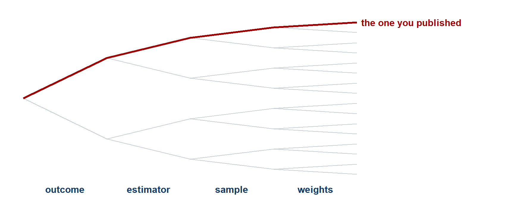
Four binary choices give sixteen analyses. Fourteen axes with several options each give hundreds of thousands. The published paper reports one red line and no tree.

Here is the structure of the problem, drawn. Four choices, two options each, and you already have sixteen distinct analyses. Our menu has fourteen axes and half of them have more than two options, which is how you get from sixteen to hundreds of thousands. The red line is what a published paper reports, one route through this tree with no indication that the tree exists. The reader sees a coefficient and a standard error, and the standard error describes uncertainty from sampling – it contains no information about the fifteen other branches. Gelman and Loken’s phrase for this is the garden of forking paths, and their sharp observation, which we met earlier, is that you do not have to walk every path for this to be a problem. Walking one path that you chose after seeing the data is enough.

Filters for inclusion

Two filters decide which of the analyses you could run go into a multiverse:

• Justifiability – could you defend this specification to a reviewer, in writing, before seeing its result?
• The same estimand – does it estimate the quantity you said you were after?

Drop the first filter and you get a cloud of nonsense that makes any finding look fragile. Drop the second and you are averaging over answers to different questions – which is the red-card mistake, at scale.

Our grid is a curated 840, chosen against both filters. That curation is itself an analytical decision, and it is the one that a critic should attack first.

This is where multiverse analysis is most often done badly, so it is worth slowing down. A multiverse is not every analysis you could run. Two filters have to be applied before a specification is allowed in. The first is justifiability: could you defend this specification to a reviewer, in writing, before seeing what it gives? The second is that it has to estimate the same quantity you said you were after. Drop the first filter and you generate a cloud of nonsense, and since nonsense specifications produce scattered answers, any finding on earth looks fragile. Drop the second and you are averaging over answers to different questions, which is the red-card mistake reproduced at scale. Our grid is a curated eight hundred and forty, chosen against both filters. And notice that the curation is itself an analytical decision – it is the first thing that a critic should attack.

Enumeration and curation

Enumerate

Cross every option on every axis. Complete, mechanical, reproducible.

Risk: the set fills up with specifications nobody would defend, and the spread stops meaning anything.

Curate

Include only the specifications you would actually defend.

Risk: you are choosing the set, so a sceptic can ask whether you chose it to get the picture you wanted.

Either way, the set is a claim, and it belongs in the paper alongside the curve, ideally preregistered before the curve is drawn.

So how do you build the set? Two strategies, and both have a real cost. Enumerate: cross every option on every axis mechanically. It is complete, it is reproducible, and nobody can accuse you of hand-picking. The risk is that the set fills up with specifications nobody would defend, and once it does, the spread stops meaning anything – of course the answer varies, you included analyses that are wrong. Or curate: include only the specifications you would actually defend in print. That fixes the first problem and creates a second, because now you are choosing the set, and a sceptic can reasonably ask whether you chose it to produce the picture you wanted. There is no way out of this dilemma, and I do not think you should pretend there is. Either way the set is a claim, it belongs in the paper next to the curve, and ideally it is preregistered before the curve is drawn.

Multiplying the menu out

Our menu, multiplied out:

• 6 outcomes × 2 predictor forms × 2 copredictor settings × 4 estimators × 5 samples × 2 weightings, minus the combinations that are not defined → 840 distinct analyses
• Add the outcome family axis → the family universe of 1,680
• Add GDP growth as the claim carrier → 2,520, the universe on the results page
• Open the four regression weights, the scoring rule, the four measurement decisions – what happens to no-opinion respondents, which items, design-weighted cells or not, which published series – and the standard-error convention → 449,280 linear specifications, 461,760 rows once the beta twins and the two imputation engines are in
• Open the unit of analysis as well – person level or aggregate – and the arithmetic doubles again

Two consequences. Compute stops being free, so somebody must decide what is worth running. And you cannot look at 450,000 numbers – you need a picture, and a way to ask which axis is doing the work.

Now multiply the menu out. Six outcomes, two predictor forms, two copredictor settings, four estimators, five samples, two weightings – minus the combinations that are not defined, like random effects with weights – and you land on eight hundred and forty distinct analyses. Add the outcome family axis and it doubles to one thousand six hundred and eighty, the family universe. Add GDP growth as an alternative claim carrier and it is two and a half thousand. Open the other regression weights, the scoring rule, the four measurement decisions and the standard-error convention, and the linear specifications alone come to four hundred and forty-nine thousand. And if you also opened the unit of analysis, person level or aggregate, the arithmetic would double again. Two consequences follow. First, compute stops being free, so somebody has to decide what is worth running, and that decision is not neutral. Second, and more practically, you cannot look at four hundred and fifty thousand numbers. You need a picture, and you need a way of asking which axis is actually doing the work.

Purposes of a multiverse

Rohrer, Hullman and Gelman’s question, and it has three different answers that need three differently built universes:

• Reflection – to understand your own analysis. Which choices matter, where the argument has to happen. Build it broad, and read it yourself
• Persuasion – to convince a reader that the finding is not an artefact of one path. Build it from specifications that your critic would accept
• Inference – to make a probabilistic statement about the curve as a whole. Build it to a rule fixed in a preregistration, and bring a null distribution

Our grid was built for reflection. Reading it as inference is a mistake that we take apart later.

Rohrer et al. (2026)

And then the question that organises the whole debate, which is Rohrer, Hullman and Gelman’s: what is a multiverse actually for? Because there are three answers and they need three differently built universes. If it is for reflection – understanding your own analysis, finding out which choices matter and where the argument has to happen – build it broad and read it yourself; it does not even have to go in the paper. If it is for persuasion – convincing a reader that your finding is not an artefact of one path – then build it out of specifications that your critic would accept, not ones you like. And if it is for inference, making a probabilistic statement about the curve as a whole, then you need a rule fixed in a preregistration and a null distribution, and that is a much heavier undertaking. Our grid was built for reflection, and reading it as inference is a mistake that we take apart later.

Decomposing the variance by fork

Once you have hundreds of estimates and the choices that produced each one, you can ask a question that no single analysis can answer: how much of the variation does each axis account for?

• Treat the specification grid as data: one row per analysis, the axes as factors, the estimate as the outcome
• Decompose the variance across axes

The answer is the most useful thing a multiverse produces, because it tells you where to spend your argument. An axis that moves nothing does not need defending, while an axis that moves everything needs a paragraph.

On this claim, the answer surprises almost everybody who guesses it in advance.

This analysis only becomes possible once you have hundreds of estimates and a record of which choices produced each one. You can turn the grid itself into a dataset – one row per analysis, the six axes of the grid of 840 as factors, the estimate as the outcome – and decompose the variance across axes. How much of the spread does each fork account for? I think that is the most useful thing a multiverse produces, and it is much more useful than the curve itself, because it tells you where to spend your argument. An axis that moves nothing does not need defending in your paper; you can say so in a sentence and move on. An axis that moves everything needs a paragraph of justification, and probably a sensitivity analysis. And on this claim the answer surprises nearly everybody who guesses it in advance.

Reading a specification curve

Five questions to ask any curve you meet, in any paper:

1. What is on the vertical axis – a raw coefficient, or something standardised? Are the signs aligned so that up and down mean the same thing throughout?
2. How was the set built – enumerated or curated, and by whom?
3. Where does the published estimate sit – at the median, or out at an end?
4. Is the spread patterned – does one axis produce the extremes, or is it scattered?
5. What null is the significance shading against – and are the specifications independent? (They almost never are.)

Answered for your own curve, the five make a publishable robustness section.

And to close the tutorial, five questions to ask of any specification curve you ever meet, in anybody’s paper. One: what is on the vertical axis – a raw coefficient, which is not comparable across outcomes, or something standardised; and are the signs aligned so that up and down mean the same thing all the way across. Two: how was the set built, enumerated or curated, and by whom. Three: where does the published estimate sit – comfortably at the median, or out at one end, because those are very different situations for the author. Four: is the spread patterned – does one axis produce all the extremes, or is it genuinely scattered. And five, the one nobody asks: what null is that significance shading against, and are the specifications independent of each other? They almost never are, and we will spend some time on why that matters. Answer all five for your own curve and you have the material for a publishable robustness section.

What the curve leaves out

• The specifications nobody ran. Person-level models, a different scale construction, a lagged predictor. The curve contains nothing from outside the menu, and looks just as complete either way
• The dependence. All 840 use the same 270 country-years, so they share their noise, and the width of the cloud cannot be read as 840 independent results
• Estimand drift. Some of these specifications answer subtly different questions. The chart puts them on one axis; that does not make them commensurable
• The data-building choices. Everything upstream of the panel – how the scales were coded, which waves were pooled – is fixed for everyone here

A curve is a map of the menu you wrote, and it cannot show whether that menu was the right one.

Four things are missing from the specification curve, and a chart as tidy as ours makes it easy to think it is complete. First, the specifications nobody ran: person-level models, a different scale construction, a lagged predictor. The curve contains nothing from outside the menu, and it looks just as complete either way, which is what makes this easy to miss. Second, the dependence: all eight hundred and forty of these use the same two hundred and seventy country-years, so they share their noise, and the width of that cloud cannot be read as eight hundred and forty independent results. Third, estimand drift: some of these answer subtly different questions, and putting them on one axis does not make them commensurable. And fourth, everything upstream of the panel – how the scales were coded, which waves were pooled – is fixed for everyone in this class. A curve is a map of the menu you wrote, and it cannot show whether the menu was right.

Description and inference

Description – map how the estimate moves across every defensible choice. (What our curve does.)

Inference – ask whether the curve as a whole is surprising if there were no effect at all. (A different, harder job.)

The two are detachable, and most published curves stop at description.

Steegen et al. (2016); Simonsohn et al. (2020)

A curve like ours does two different jobs. The first is description, showing how the estimate moves as the choices move. That is what we built, and it is useful on its own. The second is inference: asking whether the curve, taken as a whole, is more extreme than you would expect if there were no effect at all. Those are different questions with different machinery, and they detach cleanly – Multi100 did the description without the inference, and so far we have done the same. The next three slides are about what the second job takes.

Dependence among the 840 estimates

Every specification re-uses the same 270 country-years. The estimates are deeply dependent.

63.9% significant describes the curve. It is not a p-value for the claim.

Vote-counting across dependent specifications has no null distribution, so a tally of significant results is not evidence for the claim on its own.

Sixty-three point nine per cent of our specifications are significant, and it is very tempting to read that as evidence strength: most tests pass, so the claim holds. But all eight hundred and forty specifications use the same two hundred and seventy country-years. They share the data, so they share the noise: if sampling luck pushed a handful of country-years in the direction of the claim, it pushed hundreds of specifications the same way at once. The percentage significant is a description of the curve, not a test of the claim. To test the claim at curve level you need to know what the whole curve would look like if there were nothing to find, and that null has to be constructed.

The permutation design

• Break the one link that the claim needs: shuffle each country’s unemployment series in time (jointly with growth), keeping everything else intact
• Refit all 840 specifications on each shuffled dataset · repeat B = 500 times
• Compare the observed curve to the 500 null curves: is ours more extreme than chance produces?

The design is worked through in your inference reading; permutation inference after Phipson and Smyth (2010).

The claim says that a country’s unemployment moves its EU framing over time. To build the null, take each country and shuffle its unemployment series in time – together with growth, so the macro side stays internally coherent – while leaving the framing data untouched. In a shuffled world the alignment between unemployment and framing is broken by construction: whatever curve you get is what pure chance produces on these data with these 840 specifications. Do that five hundred times, refit the entire grid each time, and you have five hundred null curves to compare ours with. If our curve falls in the far tail of those null curves, the curve as a whole is evidence. If it falls comfortably among them, the description stands but the inference does not.

Reading a curve-level test

• With B = 500, the smallest reportable p is 2/(B+1) ≈ 0.004, a floor set by the number of draws, not a zero
• Near p = .05 the Monte-Carlo error is about ±0.01, so treat p = .04 and p = .06 as the same finding
• A DESIGN · NOT YET RUN – a curve-level test has to be fully specified before anyone runs it, and this one has not been run; today we read the design only

Discussion (2 minutes, then chat): the constrained cosmopolitan-only universe has 140 specs: 70.7% negative, 57.1% negative and significant. Strong evidence? Against what null?

Two literacy points and then you argue. First: with five hundred draws, the smallest p-value the test can report is two over five hundred and one – about point zero zero four. That is a floor set by the number of draws, not a zero, and more draws lower it at a real cost in computing time. Second: near the point-oh-five boundary the Monte-Carlo error is around plus or minus point zero one, so a permutation p of point zero four and one of point zero six count as the same finding. The badge says that this test is designed and has not been run, so what you are reading today is a plan whose result nobody yet knows, which is the position that a preregistration puts you in. Now the discussion beat. The constrained universe – cosmopolitan outcome only, 140 specifications – is 70.7 per cent negative, 57.1 per cent negative and significant. Two minutes: is that strong evidence? Against what null? Type your answer. [harvest: the sharp ones will say – we don’t know until we know what chance produces on these dependent data; that is the point.]

What stands without the test

Everything descriptive survives: the 49.7% outcome fork, the analysts’ placement, the sign-flip pattern, your dot.

Only one sentence depends on the permutation test: the curve as a whole is unlikely under no effect.

Careful reporting says which of the two layers a claim belongs to.

Most of what the grid has shown needs no permutation at all. That the outcome fork accounts for half the variance – description, stands. That the two person-level analysts bracket the range – stands. That the sign flips concentrate in the pooled estimator and the non-bailout samples – stands. Your own dot and the whole structure of the curve stand as well. The single sentence that has to wait is this curve as a whole is unlikely if there is no effect. Keeping those two layers apart in your own writing – saying which one your claim belongs to – is what inference literacy means in practice, and it puts you ahead of most published specification curves.

Archiving and registering a reanalysis

OSF, the Open Science Framework: a public repository in which data, code and registrations are timestamped and citable.

A registration is a frozen, dated snapshot of a plan. Anyone can check what you said you would do, and when.

You need no account today. We are going to read OSF the way that reviewers do.

Outside a classroom, an analysis plan is preregistered by filing it in a public registry. Everything you have worked with in this course – the dataset, my analysis script, the codebook – is kept at a permanent public address on the Open Science Framework. OSF does two jobs. It archives materials, which is the only reason you were able to stand in a real analyst’s shoes at all. And it registers plans: a registration is a frozen, timestamped snapshot of what you intend to do, filed before you do it, that nobody – including you – can quietly edit afterwards. You do not need an account for any of this today. We are going to read OSF the way a reviewer or a sceptical reader would, starting with the public record of this paper.

Three OSF addresses

osf.io/8rtwe – the archival Multi100 record: analyst C6HJR, frozen as submitted

osf.io/6zqct – the maintained fork: the script, the codebook, the course data

osf.io/h7432 – the full SCORE dossier on the EU-frames case: all the reports and their verdicts

Each of these does a different job. The first is the official archive: the Multi100 component for analyst C6HJR, frozen at the moment of submission and never touched again. That is what an archive is for, and it is also its limit, because an archive cannot be updated as a project moves on. The second address is the maintained fork, which is where the working materials are updated and where this course fetches its data from. A project that expects to keep changing usually needs both, an archive to preserve the record and a fork to keep the materials current. The third address is the one we open next: the full SCORE dossier on this paper, every reproduction report, the robustness study, the replication. It is all public, so let us go and read some of it.

The SCORE dossier

osf.io/h7432

• Find the secondary-data replication of the claim – new Eurobarometer data, N = 352,114
• Read its unemployment coefficient: the sign, the p-value
• Paste the b in chat when you have it (3 minutes)

Three minutes, everyone: open the dossier and find the replication component – the one that took the same claim to new Eurobarometer data, three hundred and fifty-two thousand person-years. Read what it found for the unemployment coefficient and paste the b into chat. [wait] There it is: plus zero point zero zero two, with a p of point zero four six. The sign flipped to positive on a third of a million observations, and the estimate is significant in the wrong direction, if only just. Keep that number in mind alongside the one specification that you will preregister in Task 5. If careful, well-powered re-runs can flip a sign, the only protection that a single analysis has is that it was preregistered before anyone knew the answer.

The Multi100 preregistration

• Multi100: 100 claims × at least 5 independent analysts, no instructions on how to analyse
• The scoring rules – same conclusion? effect size close? – were fixed and public before any result came back
• Outcome: 74% same conclusion · 34% within ±0.05 d

Aczel et al. (2026). Project: osf.io/7snkz

Multi100, the study in which you have been working as analyst no. 6, was itself preregistered. One hundred claims, five or more analysts each, complete analytical freedom. The part that had to be pinned down in advance was the judging: what counts as the same conclusion, how close is close for an effect size. Those rules went up on OSF before a single analyst’s result came back, which is why the seventy-four per cent and thirty-four per cent you met earlier mean something – nobody could move the goalposts once the results were in. [Confirm the registered-protocol wording against osf.io/7snkz before delivery – say what the registration actually fixed, not a paraphrase.]

Preregistration templates

• In your report: the AsPredicted short form, adapted for data you already hold – eight plain-language questions (on OSF: Preregistration Template from AsPredicted.org)
• The fuller tool for our job: the secondary-data template (van den Akker et al. 2021, Meta-Psychology) – 26 items, built for reanalysing data you already hold
• Both templates are in your reading

There are two templates, and the course uses one of them. The preregistration block in your report follows the AsPredicted short form: eight questions in plain language, the shortest recognised template there is, and completable in about eight minutes. But I want you to know its limits. AsPredicted was written for people who have not collected data yet. Its very first question – have any data been collected? – has, for us, the awkward answer it’s complicated, I already hold everything. There is a template built for that situation: the secondary-data preregistration template by van den Akker and colleagues, twenty-six items, with a whole section on what you already know about the data. It is in your reading list, and it is the tool that a full version of this exercise would use. Our block borrows that section and calls it the data-in-hand statement.

The eight AsPredicted questions

AsPredicted asks	Your block answers
Q1 Have data been collected?	It’s complicated – I already hold them + what I already know
Q2 Main question / hypothesis?	the claim, in your one sentence
Q3 Dependent variable?	your outcome axis
Q4 Conditions?	your choices on the other twelve axes
Q5 Analyses?	your model + your support/undermine rule
Q6 Outliers / exclusions?	your sample axis
Q7 Sample size?	N = 270 country-years, fewer if your sample or series leaves some out
Q8 Anything else?	your DAG-grounded justification

Each AsPredicted question maps onto a decision from an earlier task, which is why the block takes about eight minutes rather than forty. The claim sentence you typed in chat earlier is question two. Your outcome axis is the dependent variable, question three. Your choices on the other twelve axes are your conditions. Your sample axis is the exclusion rule. The sample size is two hundred and seventy country-years, fewer if your sample or your published series leaves some out. And the one question that AsPredicted handles badly for us, question one, you answer directly: the data exist, I hold them, and here is what I already know – including that the baseline comes out at minus three point eight zero four.

References

Aczel, Balazs, Barnabas Szaszi, Harry T. Clelland, et al. 2026. “Investigating the Analytical Robustness of the Social and Behavioural Sciences.” Nature 652 (8108): 135–42. https://doi.org/10.1038/s41586-025-09844-9.

Alipourfard, Nazanin, Beatrix Arendt, Daniel M Benjamin, et al. 2021. Systematizing Confidence in Open Research and Evidence (SCORE). 46mnb_v1. SocArXiv. https://doi.org/10.31235/osf.io/46mnb.

Auspurg, Katrin. 2025. “Robustness Is Better Assessed with a Few Thoughtful Models Than with Billions of Regressions.” Proceedings of the National Academy of Sciences 122 (43): e2521917122. https://doi.org/10.1073/pnas.2521917122.

Auspurg, Katrin, and Josef Brüderl. 2021. “Has the Credibility of the Social Sciences Been Credibly Destroyed? Reanalyzing the ‘Many Analysts, One Data Set’ Project.” Socius 7 (January): 23780231211024421. https://doi.org/10.1177/23780231211024421.

Breznau, Nate, Eike Mark Rinke, Alexander Wuttke, et al. 2022. “Observing Many Researchers Using the Same Data and Hypothesis Reveals a Hidden Universe of Uncertainty.” Proceedings of the National Academy of Sciences 119 (44): e2203150119. https://doi.org/10.1073/pnas.2203150119.

Cole, Stephen R., Robert W. Platt, Enrique F. Schisterman, et al. 2010. “Illustrating Bias Due to Conditioning on a Collider.” International Journal of Epidemiology 39 (2): 417–20. https://doi.org/10.1093/ije/dyp334.

D’Agostino McGowan, Lucy, Travis Gerke, and Malcolm Barrett. 2024. “Causal Inference Is Not Just a Statistics Problem.” Journal of Statistics and Data Science Education 32 (2): 150–55. https://doi.org/10.1080/26939169.2023.2276446.

Ganslmeier, Michael, and Tim Vlandas. 2025. “Estimating the Extent and Sources of Model Uncertainty in Political Science.” Proceedings of the National Academy of Sciences 122 (25): e2414926122. https://doi.org/10.1073/pnas.2414926122.

Gelman, Andrew, and Eric Loken. 2014. “The Statistical Crisis in Science.” American Scientist 102 (6): 460–66. https://doi.org/10.1511/2014.111.460.

Griffith, Gareth J., Tim T. Morris, Matthew J. Tudball, et al. 2020. “Collider Bias Undermines Our Understanding of COVID-19 Disease Risk and Severity.” Nature Communications 11 (1): 5749. https://doi.org/10.1038/s41467-020-19478-2.

Hernán, Miguel A., and James M. Robins. 2020. Causal Inference: What If. Chapman & Hall/CRC.

Huntington-Klein, Nick. 2021. The Effect: An Introduction to Research Design and Causality. Chapman & Hall/CRC. https://theeffectbook.net/.

Ioannidis, John P. A. 2005. “Why Most Published Research Findings Are False.” PLoS Medicine 2 (8): e124. https://doi.org/10.1371/journal.pmed.0020124.

John, Leslie K., George Loewenstein, and Drazen Prelec. 2012. “Measuring the Prevalence of Questionable Research Practices with Incentives for Truth Telling.” Psychological Science 23 (5): 524–32. https://doi.org/10.1177/0956797611430953.

Keele, Luke, Randolph T. Stevenson, and Felix Elwert. 2020. “The Causal Interpretation of Estimated Associations in Regression Models.” Political Science Research and Methods 8 (1): 1–13. https://doi.org/10.1017/psrm.2019.31.

Lakens, Daniel, Sajedeh Rasti, and Mehmet N. Tunç. 2026. There Is Only One Correct Analysis. PsyArXiv. https://osf.io/preprints/psyarxiv/hvjxf_v1/.

Leszczensky, Lars, and Tobias Wolbring. 2022. “How to Deal with Reverse Causality Using Panel Data? Recommendations for Researchers Based on a Simulation Study.” Sociological Methods & Research 51 (2): 837–65. https://doi.org/10.1177/0049124119882473.

Lundberg, Ian, Rebecca Johnson, and Brandon M. Stewart. 2021. “What Is Your Estimand? Defining the Target Quantity Connects Statistical Evidence to Theory.” American Sociological Review 86 (3): 532–65. https://doi.org/10.1177/00031224211004187.

Miske, Olivia, Anna Lou Abatayo, Mason Daley, et al. 2026. “Investigating the Reproducibility of the Social and Behavioural Sciences.” Nature 652 (8108): 126–34. https://doi.org/10.1038/s41586-026-10203-5.

Munafò, Marcus R., Brian A. Nosek, Dorothy V. M. Bishop, et al. 2017. “A Manifesto for Reproducible Science.” Nature Human Behaviour 1 (1): 0021. https://doi.org/10.1038/s41562-016-0021.

Nosek, Brian A, Timothy M Errington, Noah Haber, Theresa Stankov, and Andrew H Tyner. 2025. A Brief Glossary of Terms about Repeatability: Replicability, Robustness, and Reproducibility. mqfp4_v1. MetaArXiv. https://doi.org/10.31222/osf.io/mqfp4_v1.

Open Science Collaboration. 2015. “Estimating the Reproducibility of Psychological Science.” Science 349 (6251): aac4716. https://doi.org/10.1126/science.aac4716.

Phipson, Belinda, and Gordon K. Smyth. 2010. “Permutation P-values Should Never Be Zero: Calculating Exact P-values When Permutations Are Randomly Drawn.” Statistical Applications in Genetics and Molecular Biology 9 (1): Article 39. https://doi.org/10.2202/1544-6115.1585.

Rohrer, Julia M., Jessica Hullman, and Andrew Gelman. 2026. What’s a Multiverse Good for Anyway? PsyArXiv. https://osf.io/preprints/psyarxiv/37g29_v1/.

Sánchez-Tójar, Alfredo, Jelte M. Wicherts, and Robb Willer. 2026. “Huge Meta-Research Project Puts Claims in Social-Science Papers to the Test.” Nature 652 (8108): 39–41. https://doi.org/10.1038/d41586-026-00805-4.

Silberzahn, R., E. L. Uhlmann, D. P. Martin, et al. 2018. “Many Analysts, One Data Set: Making Transparent How Variations in Analytic Choices Affect Results.” Advances in Methods and Practices in Psychological Science 1 (3): 337–56. https://doi.org/10.1177/2515245917747646.

Simmons, Joseph P., Leif D. Nelson, and Uri Simonsohn. 2011. “False-Positive Psychology: Undisclosed Flexibility in Data Collection and Analysis Allows Presenting Anything as Significant.” Psychological Science 22 (11): 1359–66. https://doi.org/10.1177/0956797611417632.

Simonsohn, Uri, Joseph P. Simmons, and Leif D. Nelson. 2020. “Specification Curve Analysis.” Nature Human Behaviour 4 (11): 1208–14. https://doi.org/10.1038/s41562-020-0912-z.

Steegen, Sara, Francis Tuerlinckx, Andrew Gelman, and Wolf Vanpaemel. 2016. “Increasing Transparency Through a Multiverse Analysis.” Perspectives on Psychological Science 11 (5): 702–12. https://doi.org/10.1177/1745691616658637.

Teney, Céline. 2016. “Does the EU Economic Crisis Undermine Subjective Europeanization? Assessing the Dynamics of Citizens’ EU Framing Between 2004 and 2013.” European Sociological Review 32 (5): 619–33. https://doi.org/10.1093/esr/jcw008.

Tyner, Andrew H., Anna Lou Abatayo, Mason Daley, et al. 2026. “Investigating the Replicability of the Social and Behavioural Sciences.” Nature 652 (8108): 143–50. https://doi.org/10.1038/s41586-025-10078-y.

Young, Cristobal, and Erin Cumberworth. 2025. Multiverse Analysis: Computational Methods for Robust Results. Analytical Methods for Social Research. Cambridge University Press. https://doi.org/10.1017/9781009003391.

Feedback

Feedback form
(link in the chat · two minutes)

That brings us to the end. Before you go, the feedback form link is in the chat – two minutes, and what you write shapes the next delivery of this course. I will put the class multiverse on screen while you fill it in, so that you can find your dot one last time. Thank you for the work you put in. You reproduced a published result to the third decimal, wrote an estimand and a causal graph for a real published claim, explored a specification space, and then preregistered one specification before you ran it and put its result on the class chart.